update: The Python code for Logistic Regression can be forked/cloned from my Git repository. It is also available on PyPi. The relevant information in the blog-posts about Linear and Logistic Regression are also available as a Jupyter Notebook on my Git repository.

1. Introduction

One of the most important tasks in Machine Learning are the Classification tasks (a.k.a. supervised machine learning). Classification is used to make an accurate prediction of the class of entries in a test set (a dataset of which the entries have not yet been labelled) with the model which was constructed from a training set. You could think of classifying crime in the field of pre-policing, classifying patients in the health sector, classifying houses in the real-estate sector. Another field in which classification is big, is Natural Lanuage Processing (NLP). This goal of this field of science is to makes machines (computers) understand written (human) language. You could think of text categorization, sentiment analysis, spam detection and topic categorization.

For classification tasks there are three widely used algorithms; the Naive Bayes, Logistic Regression / Maximum Entropy and Support Vector Machines.  We have already seen how the Naive Bayes works in the context of Sentiment Analysis. Although it is more accurate than a bag-of-words model, it has the assumption of conditional independence of its features. This is a simplification which makes the NB classifier easy to implement, but it is also unrealistic in most cases and leads to a lower accuracy. A direct improvement on the N.B. classifier, is an algorithm which does not assume conditional independence but tries to estimate the weight vectors (feature values) directly. This algorithm is called Maximum Entropy in the field of NLP and Logistic Regression in the field of Statistics.

Maximum Entropy might sound like a difficult concept, but actually it is not. It is a simple idea, which can be implemented with a few lines of code. But to fully understand it, we must first go into the basics of Regression and Logistic Regression.

 

2. Regression Analysis

Regression Analysis is the field of mathematics where the goal is to find a function which best correlates with a dataset. Let’s say we have a dataset containing datapoints; . For each of these (input) datapoints there is a corresponding (output) -value. Here, the -datapoints are called the independent variables and the dependent variable; the value of depends on the value of , while the value of may be freely chosen without any restriction imposed on it by any other variable.
The goal of Regression analysis is to find a function which can best describe the correlation between and . In the field of Machine Learning, this function is called the hypothesis function and is denoted as .

 

 

If we can find such a function, we can say we have successfully built a Regression model. If the input-data lives in a 2D-space, this boils down to finding a curve which fits through the data points. In the 3D case we have to find a plane and in higher dimensions a hyperplane.

To give an example, let’s say that we are trying to find a predictive model for the success of students in a course called Machine Learning. We have a dataset which contains the final grade of  students. Dataset  contains the values of the independent variables. Our initial assumption is that the final grade only depends on the studying time. The variable therefore indicates how many hours student has studied. The first thing we would do is visualize this data:

 

 

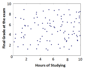
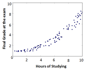
If the results looks like the figure on the left, then we are out of luck. It looks like the points are distributed randomly and there is no correlation between and at all. However, if it looks like the figure on the right, there is probably a strong correlation and we can start looking for the function which describes this correlation.

 

This function could for example be:

or

where are the dependent parameters of our model.

 

2.1. Multivariate Regression

In evaluating the results from the previous section, we may find the results unsatisfying; the function does not correlate with the datapoints strongly enough. Our initial assumption is probably not complete. Taking only the studying time into account is not enough. The final grade does not only depend on the studying time, but also on how much the students have slept the night before the exam. Now the dataset contains an additional variable which represents the sleeping time. Our dataset is then given by . In this dataset indicates how many hours student has studied and indicates how many hours he has slept.

 

This is an example of multivariate regression. The function has to include both variables. For example:

or

.

 

2.2. Linear vs Non-linear

All of the above examples are examples of linear regression. We have seen that in some cases depends on a linear form of , but it can also depend on some power of , or on the log or any other form of . However, in all cases the parameters were linear.

So, what makes linear regression linear is not that depends in a linear way on , but that it depends in a linear way on . needs to be linear with respect to the model-parameters . Mathematically speaking it needs to satisfy the superposition principle.  Examples of nonlinear regression would be:

or

 

The reason why the distinction is made between linear and nonlinear regression is that nonlinear regression problems are more difficult to solve and therefore more computational intensive algorithms are needed.
Linear regression models can be written as a linear system of equations, which can be solved by finding the closed-form solution with Linear Algebra. See these statistics notes for more on solving linear models with linear algebra.

As discussed before, such a closed-form solution can only be found for linear regression problems. However, even when the problem is linear in nature, we need to take into account that calculating the inverse of a by matrix has a time-complexity of . This means that for large datasets ( ) finding the closed-form solution will take more time than solving it iteratively (gradient descent method) as is done for nonlinear problems. So solving it iteratively is usually preferred for larger datasets, even if it is a linear problem.

 

2.3. Gradient Descent

The Gradient Descent method is a general optimization technique in which we try to find the value of the parameters with an iterative approach.
First, we construct a cost function (also known as loss function or error function) which gives the difference between the values of (the values you expect to have with the determined values of ) and the actual values of . The better your estimation of is, the better the values of will approach the values of .
Usually, the cost function is expressed as the squared error between this difference:

 

At each iteration we choose new values for the parameters , and move towards the ‘true’ values of these parameters, i.e. the values which make this cost function as small as possible. The direction in which we have to move is the negative gradient direction;

.

The reason for this is that  a function’s value decreases the fastest if we move towards the direction of the negative gradient (the directional derivative is maximal in the direction of the gradient).

Taking all this into account, this is how gradient descent works:

• Make an initial but intelligent guess for the values of the parameters .
• Keep iterating while the value of the cost function has not met your criteria:
  • With the current values of , calculate the gradient of the cost function J  ( ).
  • Update the values for the parameters 
  • Fill in these new values in the hypothesis function and calculate again the value of the cost function;

Just as important as the initial guess of the parameters is the value you choose for the learning rate . This learning rate determines how fast you move along the slope of the gradient. If the selected value of this learning rate is too small, it will take too many iterations before you reach your convergence criteria. If this value is too large, you might overshoot and not converge.

 

 

3. Logistic Regression

Logistic Regression is similar to (linear) regression, but adapted for the purpose of classification. The difference is small; for Logistic Regression we also have to apply gradient descent iteratively to estimate the values of the parameter . And again, during the iteration, the values are estimated by taking the gradient of the cost function. And again, the cost function is given by the squared error of the difference between the hypothesis function and . The major difference however, is the form of the hypothesis function.

When you want to classify something, there are a limited number of classes it can belong to. And for each of these possible classes there can only be two states for ;
either belongs to the specified class and , or it does not belong to the class and . Even though the output values are binary, the independent variables are still continuous. So, we need a function which has as input a large set of continuous variables and for each of these variables produces a binary output. This function, the hypothesis function, has the following form:

.

This function is also known as the logistic function, which is a part of the sigmoid function family. These functions are widely used in the natural sciences because they provide the simplest model for population growth. However, the reason why the logistic function is used for classification in Machine Learning is its ‘S-shape’.

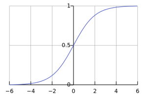
As you can see this function is bounded in the y-direction by 0 and 1. If the variable is very negative, the output function will go to zero (it does not belong to the class). If the variable  is very positive, the output will be one and it does belong to the class. (Such a function is called an indicator function.)

The question then is, what will happen to input values which are neither very positive nor very negative, but somewhere ‘in the middle’. We have to define a decision boundary, which separates the positive from the negative class. Usually this decision boundary is chosen at the middle of the logistic function, namely at where the output value is .

(1)  

For those who are wondering where entered the picture that we were talking about before. As we can see in the formula of the logistic function, . Meaning, the dependent parameter (also known as the feature), maps the input variable  to a position on the -axis. With its -value,  we can use the logistic function to calculate the -value. If this -value we assume it does belong in this class and vice versa.

So the feature should be chosen such that it predicts the class membership correctly. It is therefore essential to know which features are useful for the classification task. Once the appropriate features are selected , gradient descent can be used to find the optimal value of these features.

How can we do gradient descent with this logistic function? Except for the hypothesis function having a different form, the gradient descent method is exactly the same. We again have a cost function, of which we have to iteratively take the gradient w.r.t. the feature and update the feature value at each iteration.

This cost function is given by

 

(2)  

 

We know that:

and

(3)  

Plugging these two equations back into the cost function gives us:

(4)  

 

The gradient of the cost function with respect to is given by

(5)  

 

So the gradient of the seemingly difficult cost function, turns out to be a much simpler equation. And with this simple equation, gradient descent for Logistic Regression is again performed in the same way:

• Make an initial but intelligent guess for the values of the parameters .
• Keep iterating while the value of the cost function has not met your criteria:
  • With the current values of , calculate the gradient of the cost function J  ( ).
  • Update the values for the parameters 
  • Fill in these new values in the hypothesis function and calculate again the value of the cost function;

 

4. Text Classification and Sentiment Analysis

In the previous section we have seen how we can use Gradient Descent to estimate the feature values , which can then be used to determine the class with the Logistic function. As stated in the introduction, this can be used for a wide variety of classification tasks. The only thing that will be different for each of these classification tasks is the form the features take on.

Here we will continue to look at the example of Text Classification; Lets assume we are doing Sentiment Analysis and want to know whether a specific review should be classified as positive, neutral or negative.

The first thing we need to know is which and what types of features we need to include.
For NLP we will need a large number of features; often as large as the number of words present in the training set. We could reduce the number of features by excluding stopwords, or by only considering n-gram features.
For example, the 5-gram ‘kept me reading and reading’ is much less likely to occur in a review-document than the unigram ‘reading’, but if it occurs it is much more indicative of the class (positive) than ‘reading’. Since we only need to consider n-grams which actually are present in the training set, there will be much less features if we only consider n-grams instead of unigrams.
The second thing we need to know is the actual value of these features. The values are learned by initializing all features to zero, and applying the gradient descent method using the labeled examples in the training set. Once we know the values for the features, we can compute the probability for each class and choose the class with the maximum probability.  This is done with the following Logistic function.

 

 

5. Final Words

In this post we have discussed only the theory of Maximum Entropy and Logistic Regression. Usually such discussions are better understood with examples and the actual code. I will save that for the next blog.

If you have enjoyed reading this post or maybe even learned something from it, subscribe to this blog so you can receive a notification the next time something is posted.

 

 

6. References:

Miles Osborne, Using Maximum Entropy for Sentence Extraction (2002)

Jurafsky and Martin, Speech and Language Processing; Chapter 7

Nigam et. al., Using Maximum Entropy for Text Classification