Introduction
In the previous blog posts we have seen how we can build Convolutional Neural Networks in Tensorflow and also how we can use Stochastic Signal Analysis techniques to classify signals and time-series. In this blog post, lets have a look and see how we can build Recurrent Neural Networks in Tensorflow and use them to classify Signals.
1. Introduction to Recurrent Neural Networks
Recurrent Neural Nets (RNN) detect features in sequential data (e.g. time-series data). Examples of applications which can be made using RNN’s are anomaly detection in time-series data, classification of ECG and EEG data, stock market prediction, speech recogniton, sentiment analysis, etc.
This is done by unrolling the data into N different copies of itself (if the data consists of N time-steps) .
In this way, the input data at the previous time steps can be used when the data at timestep
is evaluated. If the data at the previous time steps is somehow correlated to the data at the current time step, these correlations are remembered and otherwise they are forgotten.
By unrolling the data, the weights of the Neural Network are shared across all of the time steps, and the RNN can generalize beyond the example seen at the current timestep, and beyond sequences seen in the training set.
This is a very short description of how an RNN works. For people who want to know more, here is some more reading material to get you up to speed. For now, what I would like you to remember is that Recurrent Neural Networks can learn whether there are temporal dependencies in the sequential data, and if there are, which dependencies / features can be used to classify the data. A RNN therefore is ideal for the classification of time-series, signals and text documents.
So, Lets start with implementing RNN’s in Tensorflow and using them to classify signals.
2. Loading the Data
This blog we will work with the CPU-friendly Human Activity Recognition Using Smartphones dataset. This dataset contains measurements done by 30 people between the ages of 19 to 48. These people have a smartphone placed on the waist while doing one of the following six activities:
- walking,
- walking upstairs,
- walking downstairs,
- sitting,
- standing or
- laying.
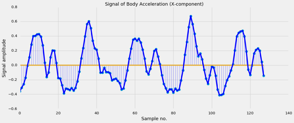
During these activities, sensor data is recorded at a constant rate of 50Hz. The signals are cut in fixed-width windows of 2.56 sec with 50% overlap. Since, these signals of 2.56 sec long have a sampling rate of 50 Hz, they will have 128 samples in total. For an illustration of this, see Figure 1a.
The smartphone measures three-axial linear body acceleration, three-axial linear total acceleration and three-axial angular velocity. So per measurement, the signal has nine components in total (see Figure 1b).
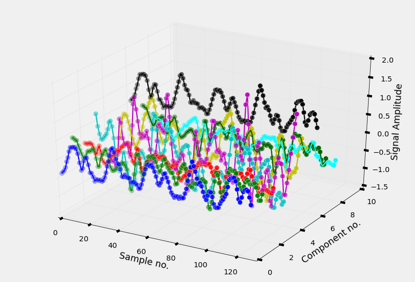
The dataset is already splitted into a training and a test part, so we can immediately load the signal into two different numpy ndarrays containing the training part and test part.
|
1 2 3 4 5 6 7 8 9 10 11 12 13 14 15 16 17 18 19 20 21 22 23 24 25 26 27 28 29 30 31 32 33 34 35 36 37 38 39 40 41 42 43 44 45 46 47 48 49 50 51 52 53 54 55 56 57 58 59 60 61 62 63 64 65 66 |
def read_signals(filename): with open(filename, 'r') as fp: data = fp.read().splitlines() data = map(lambda x: x.rstrip().lstrip().split(), data) data = [list(map(float, line)) for line in data] data = np.array(data, dtype=np.float32) return data def read_labels(filename): with open(filename, 'r') as fp: activities = fp.read().splitlines() activities = list(map(int, activities)) return np.array(activities) def randomize(dataset, labels): permutation = np.random.permutation(labels.shape[0]) shuffled_dataset = dataset[permutation, :, :] shuffled_labels = labels[permutation] return shuffled_dataset, shuffled_labels def one_hot_encode(np_array, num_labels): return (np.arange(num_labels) == np_array[:,None]).astype(np.float32) def reformat_data(dataset, labels): no_labels = len(np.unique(labels)) labels = one_hot_encode(labels, no_labels) dataset, labels = randomize(dataset, labels) return dataset, labels #### INPUT_FOLDER_TRAIN = './UCI_HAR/train/InertialSignals/' INPUT_FOLDER_TEST = './UCI_HAR/test/InertialSignals/' INPUT_FILES_TRAIN = ['body_acc_x_train.txt', 'body_acc_y_train.txt', 'body_acc_z_train.txt', 'body_gyro_x_train.txt', 'body_gyro_y_train.txt', 'body_gyro_z_train.txt', 'total_acc_x_train.txt', 'total_acc_y_train.txt', 'total_acc_z_train.txt'] INPUT_FILES_TEST = ['body_acc_x_test.txt', 'body_acc_y_test.txt', 'body_acc_z_test.txt', 'body_gyro_x_test.txt', 'body_gyro_y_test.txt', 'body_gyro_z_test.txt', 'total_acc_x_test.txt', 'total_acc_y_test.txt', 'total_acc_z_test.txt'] ##### train_signals, test_signals = [], [] for input_file in INPUT_FILES_TRAIN: signal = read_signals(INPUT_FOLDER_TRAIN + input_file) train_signals.append(signal) train_signals = np.transpose(np.array(train_signals), (1, 2, 0)) for input_file in INPUT_FILES_TEST: signal = read_signals(INPUT_FOLDER_TEST + input_file) test_signals.append(signal) test_signals = np.transpose(np.array(test_signals), (1, 2, 0)) ##### LABELFILE_TRAIN = './UCI_HAR/train/y_train.txt' LABELFILE_TEST = './UCI_HAR/test/y_test.txt' train_labels = read_labels(LABELFILE_TRAIN) test_labels = read_labels(LABELFILE_TEST) ##### train_dataset, train_labels = reformat_data(train_signals, train_labels) test_dataset, test_labels = reformat_data(test_signals, test_labels) |
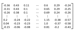
The number of signals in the training set is 7352, and the number of signals in the test set is 2947. As we can see in Figure 2, each signal has a length of of 128 samples and 9 different components, so numerically it can be considered as an array of size 128 x 9.
3. Recurrent Neural Networks in Tensorflow
As we have also seen in the previous blog posts, our Neural Network consists of a tf.Graph() and a tf.Session(). The tf.Graph() contains all of the computational steps required for the Neural Network, and the tf.Session is used to execute these steps.
The computational steps defined in the tf.Graph can be divided into four main parts;
- We initialize placeholders which are filled with batches of training data during the run.
- We define the RNN model and to calculate the output values (logits)
- The logits are used to calculate a loss value, which then
- is used in an Optimizer to optimize the weights of the RNN.
|
1 2 3 4 5 6 7 8 9 10 11 12 13 14 15 16 17 18 19 20 21 22 23 24 25 26 27 28 29 30 31 32 33 34 35 36 37 38 39 40 41 42 43 44 45 46 47 48 49 50 51 52 53 54 55 56 57 58 59 60 61 62 63 64 |
num_units = 50 signal_length = 128 num_components = 9 num_labels = 6 num_hidden = 32 learning_rate = 0.001 lambda_loss = 0.001 total_steps = 5000 display_step = 500 batch_size = 100 def accuracy(y_predicted, y): return (100.0 * np.sum(np.argmax(y_predicted, 1) == np.argmax(y, 1)) / y_predicted.shape[0]) #### graph = tf.Graph() with graph.as_default(): #1) First we put the input data in a tensorflow friendly form. tf_dataset = tf.placeholder(tf.float32, shape=(None, signal_length, num_components)) tf_labels = tf.placeholder(tf.float32, shape = (None, num_labels)) #2) Then we choose the model to calculate the logits (predicted labels) # We can choose from several models: logits = rnn_model(tf_dataset, num_hidden, num_labels) #logits = lstm_rnn_model(tf_dataset, num_hidden, num_labels) #logits = bidirectional_lstm_rnn_model(tf_dataset, num_hidden, num_labels) #logits = twolayer_lstm_rnn_model(tf_dataset, num_hidden, num_labels) #logits = gru_rnn_model(tf_dataset, num_hidden, num_labels) #3) Then we compute the softmax cross entropy between the logits and the (actual) labels l2 = lambda_loss * sum(tf.nn.l2_loss(tf_var) for tf_var in tf.trainable_variables()) loss = tf.reduce_mean(tf.nn.softmax_cross_entropy_with_logits(logits=logits, labels=tf_labels)) + l2 #4. # The optimizer is used to calculate the gradients of the loss function optimizer = tf.train.AdamOptimizer(learning_rate).minimize(loss) #optimizer = tf.train.GradientDescentOptimizer(learning_rate).minimize(loss) #optimizer = tf.train.AdagradOptimizer(learning_rate).minimize(loss) # Predictions for the training, validation, and test data. prediction = tf.nn.softmax(logits) with tf.Session(graph=graph) as session: tf.global_variables_initializer().run() print("\nInitialized") for step in range(total_steps): #Since we are using stochastic gradient descent, we are selecting small batches from the training dataset, #and training the convolutional neural network each time with a batch. offset = (step * batch_size) % (train_labels.shape[0] - batch_size) batch_data = train_dataset[offset:(offset + batch_size), :, :] batch_labels = train_labels[offset:(offset + batch_size), :] feed_dict = {tf_dataset : batch_data, tf_labels : batch_labels} _, l, train_predictions = session.run([optimizer, loss, prediction], feed_dict=feed_dict) train_accuracy = accuracy(train_predictions, batch_labels) if step % display_step == 0: feed_dict = {tf_dataset : test_dataset, tf_labels : test_labels} _, test_predictions = session.run([loss, prediction], feed_dict=feed_dict) test_accuracy = accuracy(test_predictions, test_labels) message = "step {:04d} : loss is {:06.2f}, accuracy on training set {} %, accuracy on test set {:02.2f} %".format(step, l, train_accuracy, test_accuracy) print(message) |
|
1 2 3 4 5 6 7 8 9 10 11 |
Initialized step 0000 : loss is 001.96, accuracy on training set 16.0 %, accuracy on test set 27.99 % step 0500 : loss is 000.75, accuracy on training set 60.0 %, accuracy on test set 60.67 % step 1000 : loss is 000.52, accuracy on training set 74.0 %, accuracy on test set 68.68 % step 1500 : loss is 000.66, accuracy on training set 70.0 %, accuracy on test set 69.22 % step 2000 : loss is 001.14, accuracy on training set 60.0 %, accuracy on test set 50.93 % step 2500 : loss is 001.00, accuracy on training set 74.0 %, accuracy on test set 65.97 % step 3000 : loss is 001.25, accuracy on training set 69.0 %, accuracy on test set 65.93 % step 3500 : loss is 001.40, accuracy on training set 79.0 %, accuracy on test set 69.66 % step 4000 : loss is 001.69, accuracy on training set 74.0 %, accuracy on test set 70.44 % step 4500 : loss is 002.00, accuracy on training set 77.0 %, accuracy on test set 70.68 % |
As you can see, there are different RNN Models and optimizers to choose from.
GradientDescentOptimizer is a vanilla (simple) implementation of Stochastic Gradient Descent while other implementations like the AdaOptimizer, MomentumOptimizer and AdamOptimizer dynamically adapt the learning rate to the parameters resulting in a more computational intensive process with better results. For a good explanation of the differences between all the different optimizers, have a look at Sebastian Ruders’ blog.
Besides the different types of optimizers, Tensorflow also contains different flavours of RNN’s.
We can choose from different types of cells and wrappers use them to reconstruct different types of Recurrent Neural Networks.
The basic types of cells are a BasicRNNCell, GruCell, LSTMCell, MultiRNNCell, These can be placed inside a static_rnn, dynamic_rnn or a static_bidirectional_rnn container.
In Figure 3 we can see (on the left side) a schematic overview of the process-steps of constructing a RNN Model together with (on the right side) the lines of code accompanying these steps.
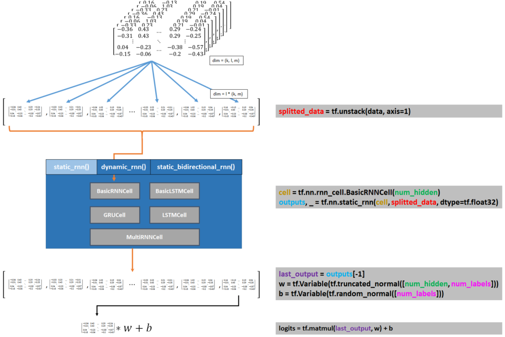
As you can see, we first split the data into a list of N different arrays with tf.unstack(). Then the type of cell is chosen and passed into the recurrent neural network together with the splitted data.
Now that we have schematically seen how we can create a RNN model, lets have a look at how we can create the different types of models in more detail.
3.1 Building the model for a RNN
Above, we have seen what the computational steps of the Neural Network consists of. But we have not yet seen the contents of our rnn_model, lstm_rnn_model, bidirectional_lstm_rnn_model, twolayer_lstm_rnn_model or gru_rnn_model. Lets have a look at how these models are constructed in more detail in the few sections below.
|
1 2 3 4 5 6 7 8 9 10 11 12 |
def rnn_model(data, num_hidden, num_labels): splitted_data = tf.unstack(data, axis=1) cell = tf.nn.rnn_cell.BasicRNNCell(num_hidden) outputs, current_state = tf.nn.static_rnn(cell, splitted_data, dtype=tf.float32) output = outputs[-1] w_softmax = tf.Variable(tf.truncated_normal([num_hidden, num_labels])) b_softmax = tf.Variable(tf.random_normal([num_labels])) logit = tf.matmul(output, w_softmax) + b_softmax return logit |
As you can see, we first split the Tensor containing the data (size batch_size, 128, 9) into a list of 128 Tensors of size (batch_size, 9) each. This is used, together with BasicRNNCell as an input for the static_rnn, which gives us a list of outputs (also of length 128).
The last output in this list (the last time step) contains information from all previous timesteps, so this is the output we will use to classify this signal.
BasicRNNCell is the most basic and vanille cell present in Tensorflow. It is an basic implementation of a RNN cell and does not have an LSTM implementation like BasicLSTMCell has. The accuracy you can achieve with BasicLSTMCell therefore is higher than BasicRNNCelll.
3.2 From BasicRNNCell to BasicLSTMCell (and beyond)
Since it does not have LSTM implemented, BasicRNNCell has its limitations. Instead of a BasicRNNCell we can use a BasicLSTMCell or an LSTMCell. Both are comparable, but a LSTMCell has some additional options like peephole structures, clipping of values, etc.
|
1 2 3 4 5 6 7 8 9 10 11 12 |
def rnn_lstm_model(data, num_hidden, num_labels): splitted_data = tf.unstack(data, axis=1) cell = tf.nn.rnn_cell.BasicLSTMCell(num_hidden) outputs, current_state = tf.nn.static_rnn(cell, splitted_data, dtype=tf.float32) output = outputs[-1] w_softmax = tf.Variable(tf.truncated_normal([num_hidden, num_labels])) b_softmax = tf.Variable(tf.random_normal([num_labels])) logit = tf.matmul(output, w_softmax) + b_softmax return logit |
3.3 GruCell: A Gated Recurrent Unit Cell
Besides BasicRNNCell and BasicLSTMCell, Tensorflow also contains GruCell, which is an abstract implementation of the Gated Recurrent Unit, proposed in 2014 by Kyunghyun Cho et al.
|
1 2 3 4 5 6 7 8 9 10 11 12 |
def gru_rnn_model(data, num_hidden, num_labels): splitted_data = tf.unstack(data, axis=1) cell = tf.contrib.rnn.GRUCell(num_hidden) outputs, current_state = tf.nn.static_rnn(cell, splitted_data, dtype=tf.float32) output = outputs[-1] w_softmax = tf.Variable(tf.truncated_normal([num_hidden, num_labels])) b_softmax = tf.Variable(tf.random_normal([num_labels])) logit = tf.matmul(output, w_softmax) + b_softmax return logit |
3.4 bi-directional LSTM RNN
The vanille RNN and LSTM RNN models we have seen so far, assume that the data at a step only depend on ‘past’ events. A bidirectional LSTM RNN, assumes that the output at step
can also depend on the data at future steps. This is not so strange if you think about applications in text analytics or speech recognition: subjects often precede verbs, adjectives precede nouns and in speech recognition the meaning of current sound may depend on the meaning of the next few sounds.
To implement a bidirectional RNN, two BasicLSTMCell’s are used; the first one looks for temporal dependencies in the backward direction and the second one for dependencies in the forward direction.
|
1 2 3 4 5 6 7 8 9 10 11 12 13 |
def bidirectional_rnn_model(data, num_hidden, num_labels): splitted_data = tf.unstack(data, axis=1) lstm_cell1 = tf.nn.rnn_cell.BasicLSTMCell(num_hidden, forget_bias=1.0, state_is_tuple=True) lstm_cell2 = tf.nn.rnn_cell.BasicLSTMCell(num_hidden, forget_bias=1.0, state_is_tuple=True) outputs, _, _ = tf.nn.static_bidirectional_rnn(lstm_cell1, lstm_cell2, splitted_data, dtype=tf.float32) output = outputs[-1] w_softmax = tf.Variable(tf.truncated_normal([num_hidden*2, num_labels])) b_softmax = tf.Variable(tf.random_normal([num_labels])) logit = tf.matmul(output, w_softmax) + b_softmax return logit |
3.5 Two-layered RNN
We have seen how we can implement a bi-directional LSTM by stacking two LSTM Cells on top of each other, where the first on looks for sequential dependencies in the forward direction, and the second one in the backward direction. You could also place two LSTM cells on top of each other, simply to increase the neural network strength.
|
1 2 3 4 5 6 7 8 9 10 11 12 13 14 |
def twolayer_rnn_model(data, num_hidden, num_labels): splitted_data = tf.unstack(data, axis=1) cell1 = tf.nn.rnn_cell.BasicLSTMCell(num_hidden, forget_bias=1.0, state_is_tuple=True) cell2 = tf.nn.rnn_cell.BasicLSTMCell(num_hidden, forget_bias=1.0, state_is_tuple=True) cell = tf.nn.rnn_cell.MultiRNNCell([cell1, cell2], state_is_tuple=True) outputs, state = tf.nn.static_rnn(cell, splitted_data, dtype=tf.float32) output = outputs[-1] w_softmax = tf.Variable(tf.truncated_normal([num_hidden, num_labels])) b_softmax = tf.Variable(tf.random_normal([num_labels])) logit = tf.matmul(output, w_softmax) + b_softmax return logit |
3.6 Multi-layered RNN
In this RNN network, n layers of RNN are stacked on top of each other. The output of each layer is mapped into the input of the next layer, and this allows the RNN to hierarchically looks for temporal dependencies. With each layer the representational power of the Neural Network increases (in theory).
|
1 2 3 4 5 6 7 8 9 10 11 12 13 14 15 16 |
def multi_rnn_model(data, num_hidden, num_labels, num_cells = 4): splitted_data = tf.unstack(data, axis=1) lstm_cells = [] for ii in range(0,num_cells): lstm_cell = tf.nn.rnn_cell.BasicLSTMCell(num_hidden, state_is_tuple=True) lstm_cells.append(lstm_cell) cell = tf.nn.rnn_cell.MultiRNNCell(lstm_cells, state_is_tuple=True) outputs, state = tf.nn.static_rnn(cell, splitted_data, dtype=tf.float32) output = outputs[-1] w_softmax = tf.Variable(tf.truncated_normal([num_hidden, num_labels])) b_softmax = tf.Variable(tf.random_normal([num_labels])) logit = tf.matmul(output, w_softmax) + b_softmax return logit |
The num_layer parameter determines how many layers are used to determine the temporal dependencies in the data. The more layers you have, the higher the representation power of the RNN is.
4. Classification results
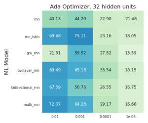
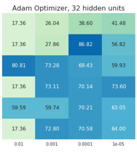
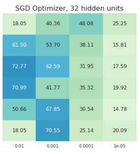
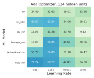
We have seen how we can build several different types of Recurrent Neural Networks. The question then is, how do these RNN’s perform in practice?
Does the accuracy really increase a lot with the number of layers or the number of hidden units?
What is the effect of the chosen optimizer and the learning rate?
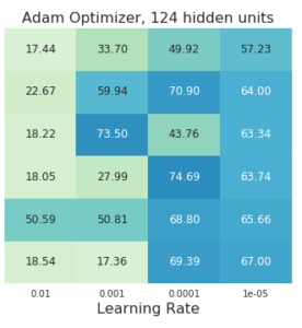
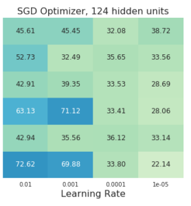
In each image you can see the final accuracy in the test set for different learning rates, models, optimizers and hidden units. You can click on each image for a more detailed graph of the training and test accuracies.
 |
 |
 |
 |
 |
 |
5. Conclusion and Final Words
In this blog-post we have seen how we can build an Recurrent Neural Network in Tensorflow, from a vanille RNN model, to an LSTM RNN, GRU RNN, bi-directional or multi-layered RNN’s. Such Recurrent Neural Networks are (powerful) tools which can be used for the analysis of time-series data or other data which is sequential in nature (like text or speech).
What I have noticed so far is:
- The most important factor to achieve high accuracy values is the chosen learning rate. It should be carefully tuned, first with large steps than with finer steps.
- AdamOptimizer usually performs best.
- More hidden units is not necessarily better. In any case, if you change the number of hidden units, you probably need to find the optimum value for learning rate again.
- For the type of RNN also; more layers is not necessarily better. BasicRNNCell has the worst performance, but except for BasicRNNCell there is no single implementation which outperforms all others in all regards. If you implement a RNN containing a BasicLSTMCell and carefully tune the learning rate and implement some l2-regularization it should be good enough for most applications.
- I am not that impressed with RNN’s in general. Same accuracy values can be / are achieved with simple stochastic analysis techniques with much less effort. With Stochastic analysis techniques you also have the benefit of knowing what the characteristic feature of each type of signal is.
[1] If you feel like you need to refresh your understanding of CNN’s, here are some good starting points to get you up to speed:
- Machine Learning is fun!
- Colah’s blog
- WildML on RNN
- DeepLearning4J on RNN
- The deeplearning book
- Some more resources
3 gedachten over “Building Recurrent Neural Networks in Tensorflow”
Hi Ahmet,
Searching the web to understand the unstacking of 3D tensors in TF I came up with your blog post. Although it helped me to solve the problem, I think that Figure 3 is wrong.
Let me explain with an example:
a = array of shape (20, 3, 2)
If unstacking with axis=1; then num = shape[axis] = shape[1] = 3.
So, as the second index gets clipped and as in the docs is stated:
Unpacks
numtensors fromvalueby chipping it along theaxisdimension. That is, we get 3 tensors of shape (20,3).So, in the image you show the tensors numbers as if they had been clipped with axis=2, which is not the case. The real image should be taking the first column of each stacked tensor (in my example, 2 columns as they are 2 stacked arrays) and building the new array as (20,2); same with all the 2nd columns and finally the same with all the 3rd columns, resulting in a list of three tensors.
I hope you understand my explanation.
Thanks for the blog post; it really helped me deeping in the notions.