In the past I have mostly written about ‘classical’ Machine Learning, like Naive Bayes classification, Logistic Regression, and the Perceptron algorithm. In the past year I have also worked with Deep Learning techniques, and I would like to share with you how to make and train a Convolutional Neural Network from scratch, using tensorflow. Later on we can use this knowledge as a building block to make interesting Deep Learning applications.
For this you will need to have tensorflow installed (see installation instructions) and you should also have a basic understanding of Python programming and the theory behind Convolutional Neural Networks. After you have installed tensorflow, you can run the smaller Neural Networks without GPU, but for the deeper networks you will definitely need some GPU power. The Internet is full with awesome websites and courses which explain how a convolutional neural network works. Some of them have good visualisations which make it easy to understand, see below. I don’t feel the need to explain the same things again, so before you continue, make sure you understand how a convolutional neural network works. For example,
- What is a convolutional layer, and what is the filter of this convolutional layer?
- What is an activation layer (ReLu layer (most widely used), sigmoid activation or tanh)?
- What is a pooling layer (max pooling / average pooling), dropout?
- How does Stochastic Gradient Descent work?
1. Tensorflow basics:
Here I will give a short introduction to Tensorflow for people who have never worked with it before. If you want to start building Neural Networks immediatly, or you are already familiar with Tensorflow you can go ahead and skip to Section 2. If you would like to know more about Tensorflow, you can also have a look at this repository, or the notes of lecture 1 and lecture 2 of Stanford’s CS20SI course.
1.1 Constants and Variables
The most basic units within tensorflow are Constants, Variables and Placeholders.
The difference between a tf.constant() and a tf.Variable() should be clear; a constant has a constant value and once you set it, it cannot be changed. The value of a Variable can be changed after it has been set, but the type and shape of the Variable can not be changed.
1
2
3
4
5
6
7
8
9
10
11
12
13
14
15
16
17
18
19
20
21
22
23
#We can create constants and variables of different types.
#However, the different types do not mix well together.
a = tf.constant(2, tf.int16)
b = tf.constant(4, tf.float32)
c = tf.constant(8, tf.float32)

d = tf.Variable(2, tf.int16)
e = tf.Variable(4, tf.float32)
f = tf.Variable(8, tf.float32)

#we can perform computations on variable of the same type: e + f
#but the following can not be done: d + e

#everything in tensorflow is a tensor, these can have different dimensions:
#0D, 1D, 2D, 3D, 4D, or nD-tensors
g = tf.constant(np.zeros(shape=(2,2), dtype=np.float32)) #does work

h = tf.zeros([11], tf.int16)
i = tf.ones([2,2], tf.float32)
j = tf.zeros([1000,4,3], tf.float64)

k = tf.Variable(tf.zeros([2,2], tf.float32))
l = tf.Variable(tf.zeros([5,6,5], tf.float32))
Besides the tf.zeros() and tf.ones(), which create a Tensor initialized to zero or one (see here), there is also the tf.random_normal() function which create a tensor filled with values picked randomly from a normal distribution (the default distribution has a mean of 0.0 and stddev of 1.0). There is also the tf.truncated_normal() function, which creates an Tensor with values randomly picked from a normal distribution, where two times the standard deviation forms the lower and upper limit.
With this knowledge, we can already create weight matrices and bias vectors which can be used in a neural network.
1
2
3
4
5
6
weights = tf.Variable(tf.truncated_normal([256 * 256, 10]))
biases = tf.Variable(tf.zeros([10]))
print(weights.get_shape().as_list())
print(biases.get_shape().as_list())
>>>[65536, 10]
>>>[10]
1.2. Tensorflow Graphs and Sessions
In Tensorflow, all of the different Variables and the operations done on these Variables are saved in a Graph. After you have build a Graph which contains all of the computational steps necessary for your model, you can run this Graph within a Session. This Session then distributes all of the computations across the available CPU and GPU resources.
1
2
3
4
5
6
7
8
9
10
11
12
13
14
graph = tf.Graph()
with graph.as_default():
    a = tf.Variable(8, tf.float32)
    b = tf.Variable(tf.zeros([2,2], tf.float32))

with tf.Session(graph=graph) as session:
    tf.global_variables_initializer().run()
    print(f)
    print(session.run(f))
    print(session.run(k))

>>> >>> 8
>>> [[ 0. 0.]
>>>  [ 0. 0.]]
1.3 Placeholders and feed_dicts
We have seen the various forms in which we can create constants and variables. Tensorflow also has placeholders; these do not require an initial value and only serve to allocate the necessary amount of memory. During a session, these placeholder can be filled in with (external) data with a feed_dict.
Below is an example of the usage of a placeholder.
1
2
3
4
5
6
7
8
9
10
11
12
13
14
15
16
17
18
19
20
21
22
23
24
25
26
27
28
29
30
31
32
33
34
35
36
list_of_points1_ = [[1,2], [3,4], [5,6], [7,8]]
list_of_points2_ = [[15,16], [13,14], [11,12], [9,10]]
list_of_points1 = np.array([np.array(elem).reshape(1,2) for elem in list_of_points1_])
list_of_points2 = np.array([np.array(elem).reshape(1,2) for elem in list_of_points2_])

graph = tf.Graph()
with graph.as_default():
    #we should use a tf.placeholder() to create a variable whose value you will fill in later (during session.run()).
    #this can be done by 'feeding' the data into the placeholder.
    #below we see an example of a method which uses two placeholder arrays of size [2,1] to calculate the eucledian distance

    point1 = tf.placeholder(tf.float32, shape=(1, 2))
    point2 = tf.placeholder(tf.float32, shape=(1, 2))

    def calculate_eucledian_distance(point1, point2):
        difference = tf.subtract(point1, point2)
        power2 = tf.pow(difference, tf.constant(2.0, shape=(1,2)))
        add = tf.reduce_sum(power2)
        eucledian_distance = tf.sqrt(add)
        return eucledian_distance

    dist = calculate_eucledian_distance(point1, point2)

with tf.Session(graph=graph) as session:
    tf.global_variables_initializer().run()
    for ii in range(len(list_of_points1)):
        point1_ = list_of_points1[ii]
        point2_ = list_of_points2[ii]
        feed_dict = {point1 : point1_, point2 : point2_}
        distance = session.run([dist], feed_dict=feed_dict)
        print("the distance between {} and {} -> {}".format(point1_, point2_, distance))

>>> the distance between [[1 2]] and [[15 16]] -> [19.79899]
>>> the distance between [[3 4]] and [[13 14]] -> [14.142136]
>>> the distance between [[5 6]] and [[11 12]] -> [8.485281]
>>> the distance between [[7 8]] and [[ 9 10]] -> [2.8284271]
2. Neural Networks in Tensorflow
2.1 Introduction
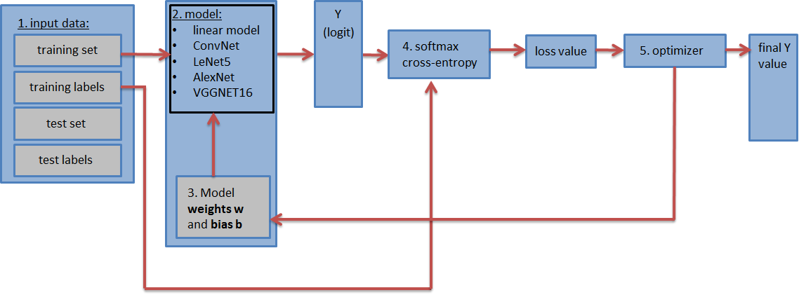
The graph containing the Neural Network (illustrated in the image above) should contain the following steps:
- The input datasets; the training dataset and labels, the test dataset and labels (and the validation dataset and labels). The test and validation datasets can be placed inside a tf.constant(). And the training dataset is placed in a tf.placeholder() so that it can be feeded in batches during the training (stochastic gradient descent).
- The Neural Network model with all of its layers. This can be a simple fully connected neural network consisting of only 1 layer, or a more complicated neural network consisting of 5, 9, 16 etc layers.
- The weight matrices and bias vectors defined in the proper shape and initialized to their initial values. (One weight matrix and bias vector per layer.)
- The loss value: the model has as output the logit vector (estimated training labels) and by comparing the logit with the actual labels, we can calculate the loss value (with the softmax with cross-entropy function). The loss value is an indication of how close the estimated training labels are to the actual training labels and will be used to update the weight values.
- An optimizer, which will use the calculated loss value to update the weights and biases with backpropagation.
2.2 Loading in the data
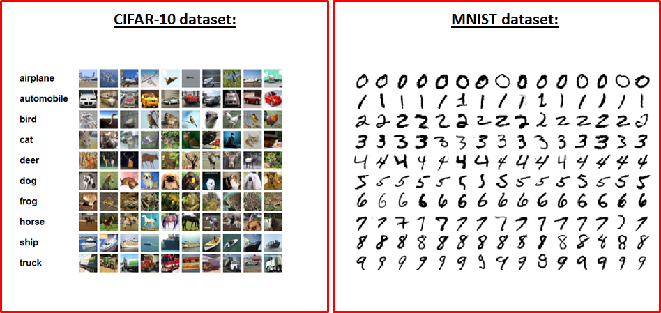
Let’s load the dataset which are going to be used to train and test the Neural Networks. For this we will download the MNIST and the CIFAR-10 dataset. The MNIST dataset contains 60.000 images of handwritten digits, where each image size is 28 x 28 x 1 (grayscale). The CIFAR-10 dataset contains 60.000 colour images (3 channels) - size 32 x 32 x 3 - of 10 different objects (airplane, automobile, bird, cat, deer, dog, frog, horse, ship, truck). Since there are 10 different objects in each dataset, both datasets contain 10 labels.
First, lets define some methods which are convenient for loading and reshaping the data into the necessary format.
1
2
3
4
5
6
7
8
9
10
11
12
13
14
15
16
17
18
19
20
21
def randomize(dataset, labels):
    permutation = np.random.permutation(labels.shape[0])
    shuffled_dataset = dataset[permutation, :, :]
    shuffled_labels = labels[permutation]
    return shuffled_dataset, shuffled_labels

def one_hot_encode(np_array):
    return (np.arange(10) == np_array[:,None]).astype(np.float32)

def reformat_data(dataset, labels, image_width, image_height, image_depth):
    np_dataset_ = np.array([np.array(image_data).reshape(image_width, image_height, image_depth) for image_data in dataset])
    np_labels_ = one_hot_encode(np.array(labels, dtype=np.float32))
    np_dataset, np_labels = randomize(np_dataset_, np_labels_)
    return np_dataset, np_labels

def flatten_tf_array(array):
    shape = array.get_shape().as_list()
    return tf.reshape(array, [shape[0], shape[1] * shape[2] * shape[3]])

def accuracy(predictions, labels):
    return (100.0 * np.sum(np.argmax(predictions, 1) == np.argmax(labels, 1)) / predictions.shape[0])
These are methods for one-hot encoding the labels, loading the data in a randomized array and a method for flattening an array (since a fully connected network needs an flat array as its input):
After we have defined these necessary function, we can load the MNIST and CIFAR-10 datasets with:
1
2
3
4
5
6
7
8
9
10
11
12
13
14
15
16
17
18
19
20
21
22
23
24
25
26
27
28
29
30
31
32
33
34
35
36
37
38
39
40
41
42
43
44
45
46
47
48
49
50
51
52
53
54
55
mnist_folder = './data/mnist/'
mnist_image_width = 28
mnist_image_height = 28
mnist_image_depth = 1
mnist_num_labels = 10

mndata = MNIST(mnist_folder)
mnist_train_dataset_, mnist_train_labels_ = mndata.load_training()
mnist_test_dataset_, mnist_test_labels_ = mndata.load_testing()

mnist_train_dataset, mnist_train_labels = reformat_data(mnist_train_dataset_, mnist_train_labels_, mnist_image_size, mnist_image_size, mnist_image_depth)
mnist_test_dataset, mnist_test_labels = reformat_data(mnist_test_dataset_, mnist_test_labels_, mnist_image_size, mnist_image_size, mnist_image_depth)

print("There are {} images, each of size {}".format(len(mnist_train_dataset), len(mnist_train_dataset[0])))
print("Meaning each image has the size of 28*28*1 = {}".format(mnist_image_size*mnist_image_size*1))
print("The training set contains the following {} labels: {}".format(len(np.unique(mnist_train_labels_)), np.unique(mnist_train_labels_)))

print('Training set shape', mnist_train_dataset.shape, mnist_train_labels.shape)
print('Test set shape', mnist_test_dataset.shape, mnist_test_labels.shape)

train_dataset_mnist, train_labels_mnist = mnist_train_dataset, mnist_train_labels
test_dataset_mnist, test_labels_mnist = mnist_test_dataset, mnist_test_labels


cifar10_folder = './data/cifar10/'
train_datasets = ['data_batch_1', 'data_batch_2', 'data_batch_3', 'data_batch_4', 'data_batch_5', ]
test_dataset = ['test_batch']
c10_image_height = 32
c10_image_width = 32
c10_image_depth = 3
c10_num_labels = 10

with open(cifar10_folder + test_dataset[0], 'rb') as f0:
    c10_test_dict = pickle.load(f0, encoding='bytes')

c10_test_dataset, c10_test_labels = c10_test_dict[b'data'], c10_test_dict[b'labels']
test_dataset_cifar10, test_labels_cifar10 = reformat_data(c10_test_dataset, c10_test_labels, c10_image_size, c10_image_size, c10_image_depth)

c10_train_dataset, c10_train_labels = [], []
for train_dataset in train_datasets:
    with open(cifar10_folder + train_dataset, 'rb') as f0:
        c10_train_dict = pickle.load(f0, encoding='bytes')
        c10_train_dataset_, c10_train_labels_ = c10_train_dict[b'data'], c10_train_dict[b'labels']

        c10_train_dataset.append(c10_train_dataset_)
        c10_train_labels += c10_train_labels_

c10_train_dataset = np.concatenate(c10_train_dataset, axis=0)
train_dataset_cifar10, train_labels_cifar10 = reformat_data(c10_train_dataset, c10_train_labels, c10_image_size, c10_image_size, c10_image_depth)
del c10_train_dataset
del c10_train_labels

print("The training set contains the following labels: {}".format(np.unique(c10_train_dict[b'labels'])))
print('Training set shape', train_dataset_cifar10.shape, train_labels_cifar10.shape)
print('Test set shape', test_dataset_cifar10.shape, test_labels_cifar10.shape)
You can download the MNIST dataset from Yann LeCun’s website. After you have downloaded and unzipped the files, you can load the data with the python-mnist tool. CIFAR-10 can be downloaded from here.
2.3 Creating a (simple) 1-layer Neural Networ
The most simple form of a Neural Network is a 1-layer linear Fully Connected Neural Network (FCNN). Mathematically it consists of a matrix multiplication. It is best to start with such a simple NN in tensorflow, and later on look at the more complicated Neural Networks. When we start looking at these more complicated Neural Networks, only the model (step 2) and weights (step 3) part of the Graph will change and the other steps will remain the same.
We can make such an 1-layer FCNN as follows:
1
2
3
4
5
6
7
8
9
10
11
12
13
14
15
16
17
18
19
20
21
22
23
24
25
26
27
28
29
30
31
32
33
34
35
36
37
38
39
40
41
42
43
44
45
46
47
48
49
50
51
52
53
54
55
56
image_width = mnist_image_width
image_height = mnist_image_height
image_depth = mnist_image_depth
num_labels = mnist_num_labels

#the dataset
train_dataset = mnist_train_dataset
train_labels = mnist_train_labels
test_dataset = mnist_test_dataset
test_labels = mnist_test_labels

#number of iterations and learning rate
num_steps = 10001
display_step = 1000
learning_rate = 0.5

graph = tf.Graph()
with graph.as_default():
    #1) First we put the input data in a tensorflow friendly form.
    tf_train_dataset = tf.placeholder(tf.float32, shape=(batch_size, image_width, image_height, image_depth))
    tf_train_labels = tf.placeholder(tf.float32, shape = (batch_size, num_labels))
    tf_test_dataset = tf.constant(test_dataset, tf.float32)

    #2) Then, the weight matrices and bias vectors are initialized
    #as a default, tf.truncated_normal() is used for the weight matrix and tf.zeros() is used for the bias vector.
    weights = tf.Variable(tf.truncated_normal([image_width * image_height * image_depth, num_labels]), tf.float32)
    bias = tf.Variable(tf.zeros([num_labels]), tf.float32)

    #3) define the model:
    #A one layered fccd simply consists of a matrix multiplication
    def model(data, weights, bias):
        return tf.matmul(flatten_tf_array(data), weights) + bias

    logits = model(tf_train_dataset, weights, bias)

    #4) calculate the loss, which will be used in the optimization of the weights
    loss = tf.reduce_mean(tf.nn.softmax_cross_entropy_with_logits(logits=logits, labels=tf_train_labels))

    #5) Choose an optimizer. Many are available.
    optimizer = tf.train.GradientDescentOptimizer(learning_rate).minimize(loss)

    #6) The predicted values for the images in the train dataset and test dataset are assigned to the variables train_prediction and test_prediction.
    #It is only necessary if you want to know the accuracy by comparing it with the actual values.
    train_prediction = tf.nn.softmax(logits)
    test_prediction = tf.nn.softmax(model(tf_test_dataset, weights, bias))

with tf.Session(graph=graph) as session:
    tf.global_variables_initializer().run()
    print('Initialized')
    for step in range(num_steps):
        _, l, predictions = session.run([optimizer, loss, train_prediction])
        if (step % display_step == 0):
            train_accuracy = accuracy(predictions, train_labels[:, :])
            test_accuracy = accuracy(test_prediction.eval(), test_labels)
            message = "step {:04d} : loss is {:06.2f}, accuracy on training set {:02.2f} %, accuracy on test set {:02.2f} %".format(step, l, train_accuracy, test_accuracy)
            print(message)
1
2
3
4
5
6
7
8
9
10
11
12
>>> Initialized
>>> step 0000 : loss is 2349.55, accuracy on training set 10.43 %, accuracy on test set 34.12 %
>>> step 0100 : loss is 3612.48, accuracy on training set 89.26 %, accuracy on test set 90.15 %
>>> step 0200 : loss is 2634.40, accuracy on training set 91.10 %, accuracy on test set 91.26 %
>>> step 0300 : loss is 2109.42, accuracy on training set 91.62 %, accuracy on test set 91.56 %
>>> step 0400 : loss is 2093.56, accuracy on training set 91.85 %, accuracy on test set 91.67 %
>>> step 0500 : loss is 2325.58, accuracy on training set 91.83 %, accuracy on test set 91.67 %
>>> step 0600 : loss is 22140.44, accuracy on training set 68.39 %, accuracy on test set 75.06 %
>>> step 0700 : loss is 5920.29, accuracy on training set 83.73 %, accuracy on test set 87.76 %
>>> step 0800 : loss is 9137.66, accuracy on training set 79.72 %, accuracy on test set 83.33 %
>>> step 0900 : loss is 15949.15, accuracy on training set 69.33 %, accuracy on test set 77.05 %
>>> step 1000 : loss is 1758.80, accuracy on training set 92.45 %, accuracy on test set 91.79 %
This is all there is too it! Inside the Graph, we load the data, define the weight matrices and the model, calculate the loss value from the logit vector and pass this to the optimizer which will update the weights for ‘num_steps’ number of iterations.
In the above fully connected NN, we have used the Gradient Descent Optimizer for optimizing the weights. However, there are many different optimizers available in tensorflow. The most common used optimizers are the GradientDescentOptimizer, AdamOptimizer and AdaGradOptimizer, so I would suggest to start with these if youre building a CNN. Sebastian Ruder has a nice blog post explaining the differences between the different optimizers which you can read if you want to know more about them.
2.4 The many faces of Tensorflow
Tensorflow contains many layers, meaning the same operations can be done with different levels of abstraction. To give a simple example, the operation logits = tf.matmul(tf_train_dataset, weights) + biases, can also be achieved with logits = tf.nn.xw_plus_b(train_dataset, weights, biases).
This is the best visible in the layers API, which is an layer with a high level of abstraction and makes it very easy to create Neural Network consisting of many different layers. For example, the conv_2d() or the fully_connected() functions create convolutional and fully connected layers. With these functions, the number of layers, filter sizes / depths, type of activation function, etc can be specified as a parameter. The weights and bias matrices are then automatically created, as well as the additional activation functions and dropout regularization layers.
For example, with the layers API, the following lines:
1
2
3
4
5
6
7
8
import tensorflow as tf

w1 = tf.Variable(tf.truncated_normal([filter_size, filter_size, image_depth, filter_depth], stddev=0.1))
b1 = tf.Variable(tf.zeros([filter_depth]))

layer1_conv = tf.nn.conv2d(data, w1, [1, 1, 1, 1], padding='SAME')
layer1_relu = tf.nn.relu(layer1_conv + b1)
layer1_pool = tf.nn.max_pool(layer1_pool, [1, 2, 2, 1], [1, 2, 2, 1], padding='SAME')
can be replaced with
1
2
3
4
from tflearn.layers.conv import conv_2d, max_pool_2d

layer1_conv = conv_2d(data, filter_depth, filter_size, activation='relu')
layer1_pool = max_pool_2d(layer1_conv_relu, 2, strides=2)
As you can see, we don’t need to define the weights, biases or activation functions. Especially when youre building a neural network with many layers, this keeps the code succint and clean.
However, if youre just starting out with tensorflow and want to learn how to build different kinds of Neural Networks, it is not ideal, since were letting tflearn do all the work. Therefore we will not use the layers API in this blog-post, but I do recommend you to use it once you have a full understanding of how a neural network should be build in tensorflow.
2.5 Creating the LeNet5 CNN
Let’s start with building more layered Neural Network. For example the LeNet5 Convolutional Neural Network.
The LeNet5 CNN architecture was thought of by Yann Lecun as early as in 1998 (see paper). It is one of the earliest CNN’s (maybe even the first?) and was specifically designed to classify handwritten digits. Although it performs well on the MNIST dataset which consist of grayscale images of size 28 x 28, the performance drops on other datasets with more images, with a larger resolution (larger image size) and more classes. For these larger datasets, deeper ConvNets (like AlexNet, VGGNet or ResNet), will perform better.
But since the LeNet5 architecture only consists of 5 layers, it is a good starting point for learning how to build CNN’s.
The Lenet5 architecture looks as follows:
As we can see, it consists of 5 layers:
- layer 1: a convolutional layer, with a sigmoid activation function, followed by an average pooling layer.
- layer 2: a convolutional layer, with a sigmoid activation function, followed by an average pooling layer.
- layer 3: a fully connected network (sigmoid activation)
- layer 4: a fully connected network (sigmoid activation)
- layer 5: the output layer
This means that we need to create 5 weight and bias matrices, and our model will consists of 12 lines of code (5 layers + 2 pooling + 4 activation functions + 1 flatten layer). Since this is quiet some code, it is best to define these in a seperate function outside of the graph.
1
2
3
4
5
6
7
8
9
10
11
12
13
14
15
16
17
18
19
20
21
22
23
24
25
26
27
28
29
30
31
32
33
34
35
36
37
38
39
40
41
42
43
44
45
46
47
48
49
LENET5_BATCH_SIZE = 32
LENET5_PATCH_SIZE = 5
LENET5_PATCH_DEPTH_1 = 6
LENET5_PATCH_DEPTH_2 = 16
LENET5_NUM_HIDDEN_1 = 120
LENET5_NUM_HIDDEN_2 = 84

def variables_lenet5(patch_size = LENET5_PATCH_SIZE, patch_depth1 = LENET5_PATCH_DEPTH_1,
                     patch_depth2 = LENET5_PATCH_DEPTH_2,
                     num_hidden1 = LENET5_NUM_HIDDEN_1, num_hidden2 = LENET5_NUM_HIDDEN_2,
                     image_depth = 1, num_labels = 10):

    w1 = tf.Variable(tf.truncated_normal([patch_size, patch_size, image_depth, patch_depth1], stddev=0.1))
    b1 = tf.Variable(tf.zeros([patch_depth1]))

    w2 = tf.Variable(tf.truncated_normal([patch_size, patch_size, patch_depth1, patch_depth2], stddev=0.1))
    b2 = tf.Variable(tf.constant(1.0, shape=[patch_depth2]))

    w3 = tf.Variable(tf.truncated_normal([5*5*patch_depth2, num_hidden1], stddev=0.1))
    b3 = tf.Variable(tf.constant(1.0, shape = [num_hidden1]))

    w4 = tf.Variable(tf.truncated_normal([num_hidden1, num_hidden2], stddev=0.1))
    b4 = tf.Variable(tf.constant(1.0, shape = [num_hidden2]))

    w5 = tf.Variable(tf.truncated_normal([num_hidden2, num_labels], stddev=0.1))
    b5 = tf.Variable(tf.constant(1.0, shape = [num_labels]))
    variables = {
        'w1': w1, 'w2': w2, 'w3': w3, 'w4': w4, 'w5': w5,
        'b1': b1, 'b2': b2, 'b3': b3, 'b4': b4, 'b5': b5
    }
    return variables

def model_lenet5(data, variables):
    layer1_conv = tf.nn.conv2d(data, variables['w1'], [1, 1, 1, 1], padding='SAME')
    layer1_actv = tf.sigmoid(layer1_conv + variables['b1'])
    layer1_pool = tf.nn.avg_pool(layer1_actv, [1, 2, 2, 1], [1, 2, 2, 1], padding='SAME')

    layer2_conv = tf.nn.conv2d(layer1_pool, variables['w2'], [1, 1, 1, 1], padding='VALID')
    layer2_actv = tf.sigmoid(layer2_conv + variables['b2'])
    layer2_pool = tf.nn.avg_pool(layer2_actv, [1, 2, 2, 1], [1, 2, 2, 1], padding='SAME')

    flat_layer = flatten_tf_array(layer2_pool)
    layer3_fccd = tf.matmul(flat_layer, variables['w3']) + variables['b3']
    layer3_actv = tf.nn.sigmoid(layer3_fccd)

    layer4_fccd = tf.matmul(layer3_actv, variables['w4']) + variables['b4']
    layer4_actv = tf.nn.sigmoid(layer4_fccd)
    logits = tf.matmul(layer4_actv, variables['w5']) + variables['b5']
    return logits
With the variables, and model defined seperately, we can adjust the the graph a little bit so that it uses these weights and model instead of the previous Fully Connected NN:
1
2
3
4
5
6
7
8
9
10
11
12
13
14
15
16
17
18
19
20
21
22
23
24
25
26
27
28
29
30
31
32
33
34
35
36
37
38
39
40
41
42
43
44
45
46
47
48
49
50
51
52
53
54
55
56
57
58
59
60
61
62
63
64
65
66
67
68
69
70
#parameters determining the model size
image_size = mnist_image_size
num_labels = mnist_num_labels

#the datasets
train_dataset = mnist_train_dataset
train_labels = mnist_train_labels
test_dataset = mnist_test_dataset
test_labels = mnist_test_labels

#number of iterations and learning rate
num_steps = 10001
display_step = 1000
learning_rate = 0.001

graph = tf.Graph()
with graph.as_default():
    #1) First we put the input data in a tensorflow friendly form.
    tf_train_dataset = tf.placeholder(tf.float32, shape=(batch_size, image_width, image_height, image_depth))
    tf_train_labels = tf.placeholder(tf.float32, shape = (batch_size, num_labels))
    tf_test_dataset = tf.constant(test_dataset, tf.float32)

    #2) Then, the weight matrices and bias vectors are initialized
    **variables = variables_lenet5(image_depth = image_depth, num_labels = num_labels)**

    #3. The model used to calculate the logits (predicted labels)
    **model = model_lenet5**
    **logits = model(tf_train_dataset, variables)**

    #4. then we compute the softmax cross entropy between the logits and the (actual) labels
    loss = tf.reduce_mean(tf.nn.softmax_cross_entropy_with_logits(logits=logits, labels=tf_train_labels))

    #5. The optimizer is used to calculate the gradients of the loss function
    optimizer = tf.train.GradientDescentOptimizer(learning_rate).minimize(loss)

    # Predictions for the training, validation, and test data.
    train_prediction = tf.nn.softmax(logits)
    test_prediction = tf.nn.softmax(model(tf_test_dataset, variables))

with tf.Session(graph=graph) as session:
    tf.global_variables_initializer().run()
    print('Initialized with learning_rate', learning_rate)
    for step in range(num_steps):

        #Since we are using stochastic gradient descent, we are selecting  small batches from the training dataset,
        #and training the convolutional neural network each time with a batch.
        offset = (step * batch_size) % (train_labels.shape[0] - batch_size)
        batch_data = train_dataset[offset:(offset + batch_size), :, :, :]
        batch_labels = train_labels[offset:(offset + batch_size), :]
        feed_dict = {tf_train_dataset : batch_data, tf_train_labels : batch_labels}
        _, l, predictions = session.run([optimizer, loss, train_prediction], feed_dict=feed_dict)

        if step % display_step == 0:
            train_accuracy = accuracy(predictions, batch_labels)
            test_accuracy = accuracy(test_prediction.eval(), test_labels)
            message = "step {:04d} : loss is {:06.2f}, accuracy on training set {:02.2f} %, accuracy on test set {:02.2f} %".format(step, l, train_accuracy, test_accuracy)
            print(message)

>>> Initialized with learning_rate 0.1
>>> step 0000 : loss is 002.49, accuracy on training set 3.12 %, accuracy on test set 10.09 %
>>> step 1000 : loss is 002.29, accuracy on training set 21.88 %, accuracy on test set 9.58 %
>>> step 2000 : loss is 000.73, accuracy on training set 75.00 %, accuracy on test set 78.20 %
>>> step 3000 : loss is 000.41, accuracy on training set 81.25 %, accuracy on test set 86.87 %
>>> step 4000 : loss is 000.26, accuracy on training set 93.75 %, accuracy on test set 90.49 %
>>> step 5000 : loss is 000.28, accuracy on training set 87.50 %, accuracy on test set 92.79 %
>>> step 6000 : loss is 000.23, accuracy on training set 96.88 %, accuracy on test set 93.64 %
>>> step 7000 : loss is 000.18, accuracy on training set 90.62 %, accuracy on test set 95.14 %
>>> step 8000 : loss is 000.14, accuracy on training set 96.88 %, accuracy on test set 95.80 %
>>> step 9000 : loss is 000.35, accuracy on training set 90.62 %, accuracy on test set 96.33 %
>>> step 10000 : loss is 000.12, accuracy on training set 93.75 %, accuracy on test set 96.76 %
As we can see the LeNet5 architecture performs better on the MNIST dataset than a simple fully connected NN.
2.6 How the parameters affect the outputsize of an layer
Generally it is true that the more layers a Neural Network has, the better it performs. We can add more layers, change activation functions and pooling layers, change the learning rate and see how each step affects the performance. Since the input of layer \(i\) is the output of layer \(i - 1\), we need to know how the output size of layer \(i -1\) is affected by its different parameters.
To understand this, lets have a look at the conv2d() function.
It has four parameters:
- The input image, a 4D Tensor with dimensions [batch size, image_width, image_height, image_depth]
- An weight matrix, a 4-D Tensor with dimensions [filter_size, filter_size, image_depth, filter_depth]
- The number of strides in each dimension.
- Padding (= ‘SAME’ / ‘VALID’)
These four parameters determine the size of the output image.
The first two parameters are the 4-D Tensor containing the batch of input images and the 4-D Tensor containing the weights of the convolutional filter.
The third parameter is the stride of the convolution, i.e. how much the convolutional filter should skip positions in each of the four dimension. The first of these 4 dimensions indicates the image-number in the batch of images and since we dont want to skip over any image, this will always be 1. The last dimension indicates the image depth (no of color-channels; 1 for grayscale and 3 for RGB) and since we dont want to skip over any color-channels, this is also always 1. The second and third dimension indicate the stride in the X and Y direction (image width and height). If we want to apply a stride, these are the dimensions in which the filter should skip positions. So for a stride of 1, we have to set the stride-parameter to [1, 1, 1, 1] and if we want a stride of 2, set it to [1, 2, 2, 1]. etc
The last parameter indicates whether or not tensorflow should zero-pad the image in order to make sure the output size does not change size for a stride of 1. With padding = ‘SAME’ the image does get zero-padded (and output size does not change), with padding = ‘VALID’ it does not.
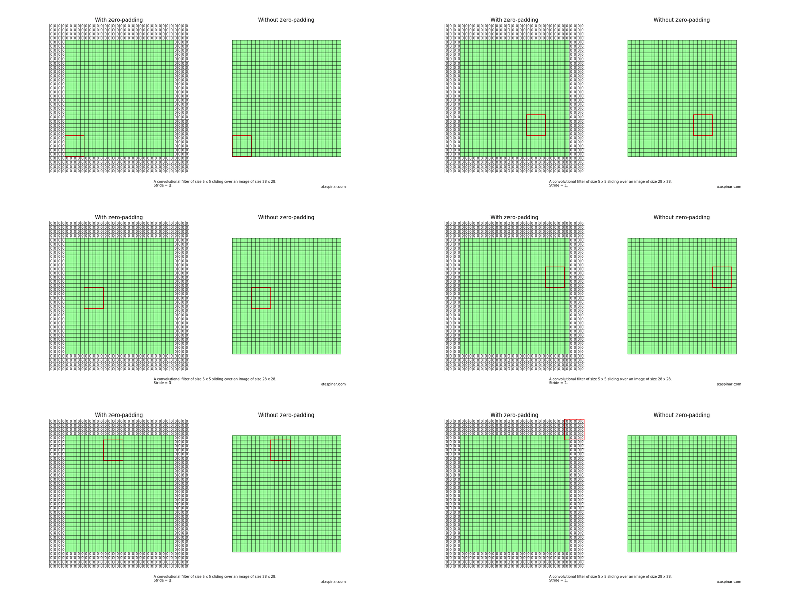
Below we can see two examples of a convolutional filter (with filter size 5 x 5) scanning through an image (of size 28 x 28). On the left the padding parameter is set to ‘SAME’, the image is zero-padded and the last 4 rows / columns are included in the output image. On the right padding is set to ‘VALID’, the image does not get zero-padded and the last 4 rows/columns are not included.
As we can see, without zero-padding the last four cells are not included, because the convolutional filter has reached the end of the (non-zero padded) image. This means that, for an input size of 28 x 28, the output size becomes 24 x 24. If padding = ‘SAME’, the output size is 28 x 28.
This becomes more clear if we write down the positions of the filter on the image while it is scanning through the image (For simplicity, only the X-direction). With a stride of 1, the X-positions are 0-5, 1-6, 2-7, etc. If the stride is 2, the X-positions are 0-5, 2-7, 4-9, etc.
If we do this for an image size of 28 x 28, filter size of 5 x 5 and strides 1 to 4, we will get the following table:
As you can see, for a stride of 1, and zero-padding the output image size is 28 x 28. Without zero-padding the output image size becomes 24 x 24. For a filter with a stride of 2, these numbers are 14 x 14 and 12 x 12, and for a filter with stride 3 it is 10 x 10 and 8 x 8. etc
For any arbitrary chosen stride S, filter size K, image size W, and padding-size P, the output size will be
\[O = 1 + (W - K + 2P) / S\]If padding = ‘SAME’ in tensorflow, the numerator always adds up to 1 and the output size is only determined by the stride S.
2.7 Adjusting the LeNet5 architecture
In the original paper, a sigmoid activation function and average pooling were used in the LeNet5 architecture. However, nowadays, it is much more common to use a relu activation function. So let’s change the LeNet5 CNN a little bit to see if we can improve its accuracy. We will call this the LeNet5-like Architecture:
1
2
3
4
5
6
7
8
9
10
11
12
13
14
15
16
17
18
19
20
21
22
23
24
25
26
27
28
29
30
31
32
33
34
35
36
37
38
39
40
41
42
43
44
45
46
47
48
49
50
LENET5_LIKE_BATCH_SIZE = 32
LENET5_LIKE_FILTER_SIZE = 5
LENET5_LIKE_FILTER_DEPTH = 16
LENET5_LIKE_NUM_HIDDEN = 120

def variables_lenet5_like(filter_size = LENET5_LIKE_FILTER_SIZE,
                          filter_depth = LENET5_LIKE_FILTER_DEPTH,
                          num_hidden = LENET5_LIKE_NUM_HIDDEN,
                          image_width = 28, image_depth = 1, num_labels = 10):

    w1 = tf.Variable(tf.truncated_normal([filter_size, filter_size, image_depth, filter_depth], stddev=0.1))
    b1 = tf.Variable(tf.zeros([filter_depth]))

    w2 = tf.Variable(tf.truncated_normal([filter_size, filter_size, filter_depth, filter_depth], stddev=0.1))
    b2 = tf.Variable(tf.constant(1.0, shape=[filter_depth]))

    w3 = tf.Variable(tf.truncated_normal([(image_width // 4)*(image_width // 4)*filter_depth , num_hidden], stddev=0.1))
    b3 = tf.Variable(tf.constant(1.0, shape = [num_hidden]))

    w4 = tf.Variable(tf.truncated_normal([num_hidden, num_hidden], stddev=0.1))
    b4 = tf.Variable(tf.constant(1.0, shape = [num_hidden]))

    w5 = tf.Variable(tf.truncated_normal([num_hidden, num_labels], stddev=0.1))
    b5 = tf.Variable(tf.constant(1.0, shape = [num_labels]))
    variables = {
                  'w1': w1, 'w2': w2, 'w3': w3, 'w4': w4, 'w5': w5,
                  'b1': b1, 'b2': b2, 'b3': b3, 'b4': b4, 'b5': b5
                }
    return variables

def model_lenet5_like(data, variables):
    layer1_conv = tf.nn.conv2d(data, variables['w1'], [1, 1, 1, 1], padding='SAME')
    layer1_actv = tf.nn.relu(layer1_conv + variables['b1'])
    layer1_pool = tf.nn.avg_pool(layer1_actv, [1, 2, 2, 1], [1, 2, 2, 1], padding='SAME')

    layer2_conv = tf.nn.conv2d(layer1_pool, variables['w2'], [1, 1, 1, 1], padding='SAME')
    layer2_actv = tf.nn.relu(layer2_conv + variables['b2'])
    layer2_pool = tf.nn.avg_pool(layer2_actv, [1, 2, 2, 1], [1, 2, 2, 1], padding='SAME')

    flat_layer = flatten_tf_array(layer2_pool)
    layer3_fccd = tf.matmul(flat_layer, variables['w3']) + variables['b3']
    layer3_actv = tf.nn.relu(layer3_fccd)
    #layer3_drop = tf.nn.dropout(layer3_actv, 0.5)

    layer4_fccd = tf.matmul(layer3_actv, variables['w4']) + variables['b4']
    layer4_actv = tf.nn.relu(layer4_fccd)
   #layer4_drop = tf.nn.dropout(layer4_actv, 0.5)

    logits = tf.matmul(layer4_actv, variables['w5']) + variables['b5']
    return logits
The main differences are that we are using a relu activation function instead of a sigmoid activation.
Besides the activation function, we can also change the used optimizers to see what the effect is of the different optimizers on accuracy.
2.8 Impact of Learning Rate and Optimizer
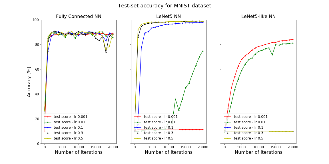
Lets see how these CNN’s perform on the MNIST and CIFAR-10 datasets.
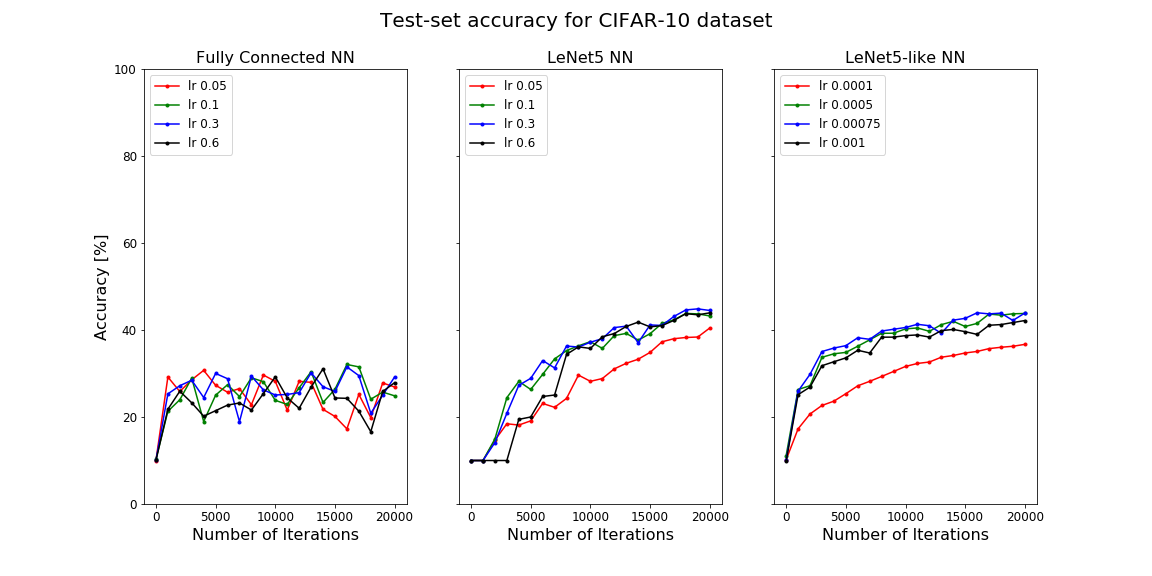
In the figures above, the accuracy on the test set is given as a function of the number of iterations. On the left for the one layer fully connected NN, in the middle for the LeNet5 NN and on the right for the LeNet5-like NN.
As we can see, the LeNet5 CNN works pretty good for the MNIST dataset. Which should not be such a big surprise, since it was specially designed to classify handwritten digits. The MNIST dataset is quiet small and does not provide a big challenge, so even a one layer fully connected network performs quiet good.
On the CIFAR-10 Dataset however, the performance for the LeNet5 NN drops significantly to accuracy values around 40%.
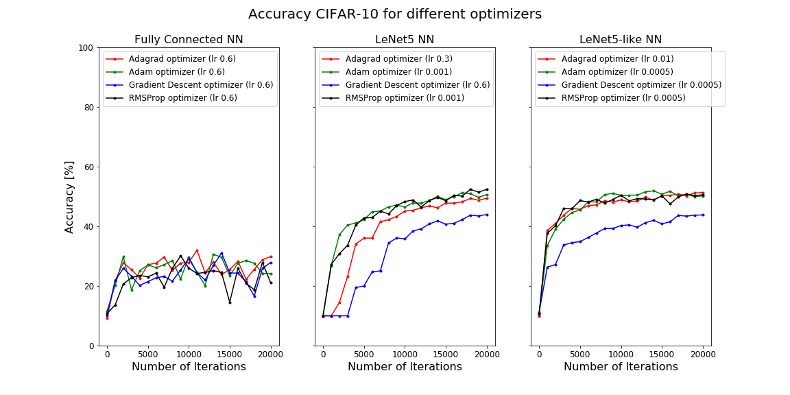
To increase the accuracy, we can change the optimizer, or fine-tune the Neural Network by applying regularization or learning rate decay.
As we can see, the AdagradOptimizer, AdamOptimizer and the RMSPropOptimizer have a better performance than the GradientDescentOptimizer. These are adaptive optimizers which in general perform better than the (simple) GradientDescentOptimizer but need more computational power.
With L2-regularization or exponential rate decay we can probably gain a bit more accuracy, but for much better results we need to go deeper.
3. Deep Neural Networks in Tensorflow
So far we have seen the LeNet5 CNN architecture. LeNet5 contains two convolutional layers followed by fully connected layers and therefore could be called a shallow Neural Network. At that time (in 1998) GPU’s were not used for computational calculations, and the CPU’s were not even that powerful so for that time the two convolutional layers were already quiet innovative.
Later on, many other types of Convolutional Neural Networks have been designed, most of them much deeper (see below for more info). There is the famous AlexNet architecture (2012) by Alex Krizhevsky et. al., the 7-layered ZF Net (2013), and the 16-layered VGGNet (2014). In 2015 Google came with 22-layered CNN with an inception module (GoogLeNet), and Microsoft Research Asia created the 152-layered CNN called ResNet.
Now, with the things we have learned so far, lets see how we can create the AlexNet and VGGNet16 architectures in Tensorflow.
3.1 AlexNet
Although LeNet5 was the first ConvNet, it is considered to be a shallow neural network. It performs well on the MNIST dataset which consist of grayscale images of size 28 x 28, but the performance drops when we’re trying to classify larger images, with more resolution and more classes.
The first Deep CNN came out in 2012 and is called AlexNet after its creators Alex Krizhevsky, Ilya Sutskever, and Geoffrey Hinton. Compared to the most recent architectures AlexNet can be considered simple, but at that time it was really succesfull. It won the ImageNet competition with a incredible test error rate of 15.4% (while the runner-up had an error of 26.2%) and started a revolution (also see this video) in the world of Deep Learning and AI.
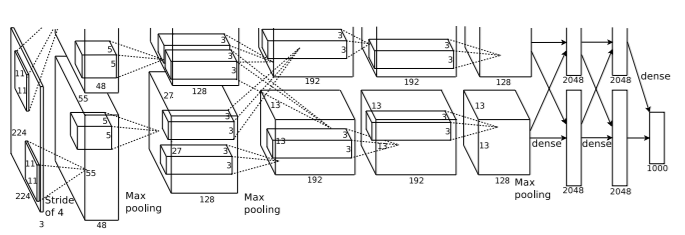
It consists of 5 convolutional layers (with relu activation), 3 max pooling layers, 3 fully connected layers and 2 dropout layers. The overall architecture looks as follows:
- layer 0: input image of size 224 x 224 x 3
- layer 1: A convolutional layer with 96 filters (filter_depth_1 = 96) of size 11 x 11 (filter_size_1 = 11) and a stride of 4. It has a relu activation function. This is followed by max pooling and local response normalization layers.
- layer 2: A convolutional layer with 256 filters (filter_depth_2 = 256) of size 5 x 5 (filter_size_2 = 5) and a stride of 1. It has a relu activation function. This layer is also followed by max pooling and local response normalization layers.
- layer 3: A convolutional layer with 384 filters (filter_depth_3 = 384) of size 3 x 3 (filter_size_3 = 3) and a stride of 1. It has a relu activation function.
- layer 4: Same as layer 3.
- layer 5: A convolutional layer with 256 filters (filter_depth_4 = 256) of size 3 x 3 (filter_size_4 = 3) and a stride of 1. It has a relu activation function.
- layer 6-8: These convolutional layers are followed by fully connected layers with 4096 neurons each. In the original paper they are classifying a dataset with 1000 classes, but we will use the oxford17 dataset, which has 17 different classes (of flowers).
Note that this CNN (or other deep CNN’s) cannot be used on the MNIST or the CIFAR-10 dataset, because the images in these datasets are too small. As we have seen before, a pooling layer (or a convolutional layer with a stride of 2) reduces the image size by a factor of 2. AlexNet has 3 max pooling layers and one convolutional layer with a stride of 4. This means that the original image size gets reduced by a factor of \(2^5\). The images in the MNIST dataset would simply get reduced to a size smaller than 0.
Therefore we need to load a dataset with larger images, preferably 224 x 224 x 3 (as the original paper indicates). The 17 category flower dataset, aka oxflower17 dataset is ideal since it contains images of exactly this size:
1
2
3
4
5
6
7
8
9
10
11
12
ox17_image_width = 224
ox17_image_height = 224
ox17_image_depth = 3
ox17_num_labels = 17

import tflearn.datasets.oxflower17 as oxflower17
train_dataset_, train_labels_ = oxflower17.load_data(one_hot=True)
train_dataset_ox17, train_labels_ox17 = train_dataset_[:1000,:,:,:], train_labels_[:1000,:]
test_dataset_ox17, test_labels_ox17 = train_dataset_[1000:,:,:,:], train_labels_[1000:,:]

print('Training set', train_dataset_ox17.shape, train_labels_ox17.shape)
print('Test set', test_dataset_ox17.shape, test_labels_ox17.shape)
Lets try to create the weight matrices and the different layers present in AlexNet. As we have seen before, we need as much weight matrices and bias vectors as the amount of layers, and each weight matrix should have a size corresponding to the filter size of the layer it belongs to.
1
2
3
4
5
6
7
8
9
10
11
12
13
14
15
16
17
18
19
20
21
22
23
24
25
26
27
28
29
30
31
32
33
34
35
36
37
38
39
40
41
42
43
44
45
46
47
48
49
50
51
52
53
54
55
56
57
58
59
60
61
62
63
64
65
66
67
68
69
70
71
72
73
74
75
76
77
ALEX_PATCH_DEPTH_1, ALEX_PATCH_DEPTH_2, ALEX_PATCH_DEPTH_3, ALEX_PATCH_DEPTH_4 = 96, 256, 384, 256
ALEX_PATCH_SIZE_1, ALEX_PATCH_SIZE_2, ALEX_PATCH_SIZE_3, ALEX_PATCH_SIZE_4 = 11, 5, 3, 3
ALEX_NUM_HIDDEN_1, ALEX_NUM_HIDDEN_2 = 4096, 4096

def variables_alexnet(patch_size1 = ALEX_PATCH_SIZE_1, patch_size2 = ALEX_PATCH_SIZE_2,
                      patch_size3 = ALEX_PATCH_SIZE_3, patch_size4 = ALEX_PATCH_SIZE_4,
                      patch_depth1 = ALEX_PATCH_DEPTH_1, patch_depth2 = ALEX_PATCH_DEPTH_2,
                      patch_depth3 = ALEX_PATCH_DEPTH_3, patch_depth4 = ALEX_PATCH_DEPTH_4,
                      num_hidden1 = ALEX_NUM_HIDDEN_1, num_hidden2 = ALEX_NUM_HIDDEN_2,
                      image_width = 224, image_height = 224, image_depth = 3, num_labels = 17):

    w1 = tf.Variable(tf.truncated_normal([patch_size1, patch_size1, image_depth, patch_depth1], stddev=0.1))
    b1 = tf.Variable(tf.zeros([patch_depth1]))

    w2 = tf.Variable(tf.truncated_normal([patch_size2, patch_size2, patch_depth1, patch_depth2], stddev=0.1))
    b2 = tf.Variable(tf.constant(1.0, shape=[patch_depth2]))

    w3 = tf.Variable(tf.truncated_normal([patch_size3, patch_size3, patch_depth2, patch_depth3], stddev=0.1))
    b3 = tf.Variable(tf.zeros([patch_depth3]))

    w4 = tf.Variable(tf.truncated_normal([patch_size4, patch_size4, patch_depth3, patch_depth3], stddev=0.1))
    b4 = tf.Variable(tf.constant(1.0, shape=[patch_depth3]))

    w5 = tf.Variable(tf.truncated_normal([patch_size4, patch_size4, patch_depth3, patch_depth3], stddev=0.1))
    b5 = tf.Variable(tf.zeros([patch_depth3]))

    pool_reductions = 3
    conv_reductions = 2
    no_reductions = pool_reductions + conv_reductions
    w6 = tf.Variable(tf.truncated_normal([(image_width // 2**no_reductions)*(image_height // 2**no_reductions)*patch_depth3, num_hidden1], stddev=0.1))
    b6 = tf.Variable(tf.constant(1.0, shape = [num_hidden1]))

    w7 = tf.Variable(tf.truncated_normal([num_hidden1, num_hidden2], stddev=0.1))
    b7 = tf.Variable(tf.constant(1.0, shape = [num_hidden2]))

    w8 = tf.Variable(tf.truncated_normal([num_hidden2, num_labels], stddev=0.1))
    b8 = tf.Variable(tf.constant(1.0, shape = [num_labels]))

    variables = {
                 'w1': w1, 'w2': w2, 'w3': w3, 'w4': w4, 'w5': w5, 'w6': w6, 'w7': w7, 'w8': w8,
                 'b1': b1, 'b2': b2, 'b3': b3, 'b4': b4, 'b5': b5, 'b6': b6, 'b7': b7, 'b8': b8
                }
    return variables

def model_alexnet(data, variables):
    layer1_conv = tf.nn.conv2d(data, variables['w1'], [1, 4, 4, 1], padding='SAME')
    layer1_relu = tf.nn.relu(layer1_conv + variables['b1'])
    layer1_pool = tf.nn.max_pool(layer1_relu, [1, 3, 3, 1], [1, 2, 2, 1], padding='SAME')
    layer1_norm = tf.nn.local_response_normalization(layer1_pool)

    layer2_conv = tf.nn.conv2d(layer1_norm, variables['w2'], [1, 1, 1, 1], padding='SAME')
    layer2_relu = tf.nn.relu(layer2_conv + variables['b2'])
    layer2_pool = tf.nn.max_pool(layer2_relu, [1, 3, 3, 1], [1, 2, 2, 1], padding='SAME')
    layer2_norm = tf.nn.local_response_normalization(layer2_pool)

    layer3_conv = tf.nn.conv2d(layer2_norm, variables['w3'], [1, 1, 1, 1], padding='SAME')
    layer3_relu = tf.nn.relu(layer3_conv + variables['b3'])

    layer4_conv = tf.nn.conv2d(layer3_relu, variables['w4'], [1, 1, 1, 1], padding='SAME')
    layer4_relu = tf.nn.relu(layer4_conv + variables['b4'])

    layer5_conv = tf.nn.conv2d(layer4_relu, variables['w5'], [1, 1, 1, 1], padding='SAME')
    layer5_relu = tf.nn.relu(layer5_conv + variables['b5'])
    layer5_pool = tf.nn.max_pool(layer4_relu, [1, 3, 3, 1], [1, 2, 2, 1], padding='SAME')
    layer5_norm = tf.nn.local_response_normalization(layer5_pool)

    flat_layer = flatten_tf_array(layer5_norm)
    layer6_fccd = tf.matmul(flat_layer, variables['w6']) + variables['b6']
    layer6_tanh = tf.tanh(layer6_fccd)
    layer6_drop = tf.nn.dropout(layer6_tanh, 0.5)

    layer7_fccd = tf.matmul(layer6_drop, variables['w7']) + variables['b7']
    layer7_tanh = tf.tanh(layer7_fccd)
    layer7_drop = tf.nn.dropout(layer7_tanh, 0.5)

    logits = tf.matmul(layer7_drop, variables['w8']) + variables['b8']
    return logits
Now we can modify the CNN model to use the weights and layers of the AlexNet model in order to classify images.
3.2 VGG Net-16
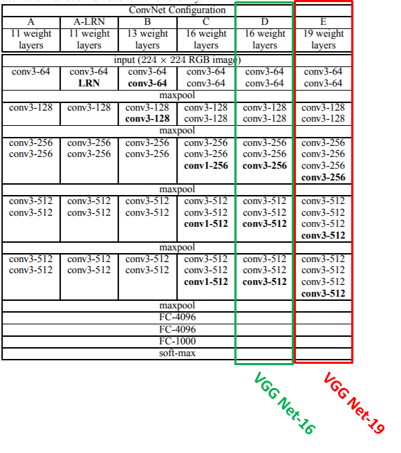
VGG Net was created in 2014 by Karen Simonyan and Andrew Zisserman of the University of Oxford. It contains much more layers (16-19 layers), but each layer is simpler in its design; all of the convolutional layers have filters of size 3 x 3 and stride of 1 and all max pooling layers have a stride of 2. So it is a deeper CNN but simpler.
It comes in different configurations, with either 16 or 19 layers. The difference between these two different configurations is the usage of either 3 or 4 convolutional layers after the second, third and fourth max pooling layer (see below).
The configuration with 16 layers (configuration D) seems to produce the best results, so lets try to create that in tensorflow.
1
2
3
4
5
6
7
8
9
10
11
12
13
14
15
16
17
18
19
20
21
22
23
24
25
26
27
28
29
30
31
32
33
34
35
36
37
38
39
40
41
42
43
44
45
46
47
48
49
50
51
52
53
54
55
56
57
58
59
60
61
62
63
64
65
66
67
68
69
70
71
72
73
74
75
76
77
78
79
80
81
82
83
84
85
86
87
88
89
90
91
92
93
94
95
96
97
98
99
100
101
102
103
104
105
106
107
108
109
#The VGGNET Neural Network
VGG16_PATCH_SIZE_1, VGG16_PATCH_SIZE_2, VGG16_PATCH_SIZE_3, VGG16_PATCH_SIZE_4 = 3, 3, 3, 3
VGG16_PATCH_DEPTH_1, VGG16_PATCH_DEPTH_2, VGG16_PATCH_DEPTH_3, VGG16_PATCH_DEPTH_4 = 64, 128, 256, 512
VGG16_NUM_HIDDEN_1, VGG16_NUM_HIDDEN_2 = 4096, 1000

def variables_vggnet16(patch_size1 = VGG16_PATCH_SIZE_1, patch_size2 = VGG16_PATCH_SIZE_2,
                       patch_size3 = VGG16_PATCH_SIZE_3, patch_size4 = VGG16_PATCH_SIZE_4,
                       patch_depth1 = VGG16_PATCH_DEPTH_1, patch_depth2 = VGG16_PATCH_DEPTH_2,
                       patch_depth3 = VGG16_PATCH_DEPTH_3, patch_depth4 = VGG16_PATCH_DEPTH_4,
                       num_hidden1 = VGG16_NUM_HIDDEN_1, num_hidden2 = VGG16_NUM_HIDDEN_2,
                       image_width = 224, image_height = 224, image_depth = 3, num_labels = 17):

    w1 = tf.Variable(tf.truncated_normal([patch_size1, patch_size1, image_depth, patch_depth1], stddev=0.1))
    b1 = tf.Variable(tf.zeros([patch_depth1]))
    w2 = tf.Variable(tf.truncated_normal([patch_size1, patch_size1, patch_depth1, patch_depth1], stddev=0.1))
    b2 = tf.Variable(tf.constant(1.0, shape=[patch_depth1]))

    w3 = tf.Variable(tf.truncated_normal([patch_size2, patch_size2, patch_depth1, patch_depth2], stddev=0.1))
    b3 = tf.Variable(tf.constant(1.0, shape = [patch_depth2]))
    w4 = tf.Variable(tf.truncated_normal([patch_size2, patch_size2, patch_depth2, patch_depth2], stddev=0.1))
    b4 = tf.Variable(tf.constant(1.0, shape = [patch_depth2]))

    w5 = tf.Variable(tf.truncated_normal([patch_size3, patch_size3, patch_depth2, patch_depth3], stddev=0.1))
    b5 = tf.Variable(tf.constant(1.0, shape = [patch_depth3]))
    w6 = tf.Variable(tf.truncated_normal([patch_size3, patch_size3, patch_depth3, patch_depth3], stddev=0.1))
    b6 = tf.Variable(tf.constant(1.0, shape = [patch_depth3]))
    w7 = tf.Variable(tf.truncated_normal([patch_size3, patch_size3, patch_depth3, patch_depth3], stddev=0.1))
    b7 = tf.Variable(tf.constant(1.0, shape=[patch_depth3]))

    w8 = tf.Variable(tf.truncated_normal([patch_size4, patch_size4, patch_depth3, patch_depth4], stddev=0.1))
    b8 = tf.Variable(tf.constant(1.0, shape = [patch_depth4]))
    w9 = tf.Variable(tf.truncated_normal([patch_size4, patch_size4, patch_depth4, patch_depth4], stddev=0.1))
    b9 = tf.Variable(tf.constant(1.0, shape = [patch_depth4]))
    w10 = tf.Variable(tf.truncated_normal([patch_size4, patch_size4, patch_depth4, patch_depth4], stddev=0.1))
    b10 = tf.Variable(tf.constant(1.0, shape = [patch_depth4]))

    w11 = tf.Variable(tf.truncated_normal([patch_size4, patch_size4, patch_depth4, patch_depth4], stddev=0.1))
    b11 = tf.Variable(tf.constant(1.0, shape = [patch_depth4]))
    w12 = tf.Variable(tf.truncated_normal([patch_size4, patch_size4, patch_depth4, patch_depth4], stddev=0.1))
    b12 = tf.Variable(tf.constant(1.0, shape=[patch_depth4]))
    w13 = tf.Variable(tf.truncated_normal([patch_size4, patch_size4, patch_depth4, patch_depth4], stddev=0.1))
    b13 = tf.Variable(tf.constant(1.0, shape = [patch_depth4]))

    no_pooling_layers = 5

    w14 = tf.Variable(tf.truncated_normal([(image_width // (2**no_pooling_layers))*(image_height // (2**no_pooling_layers))*patch_depth4 , num_hidden1], stddev=0.1))
    b14 = tf.Variable(tf.constant(1.0, shape = [num_hidden1]))

    w15 = tf.Variable(tf.truncated_normal([num_hidden1, num_hidden2], stddev=0.1))
    b15 = tf.Variable(tf.constant(1.0, shape = [num_hidden2]))

    w16 = tf.Variable(tf.truncated_normal([num_hidden2, num_labels], stddev=0.1))
    b16 = tf.Variable(tf.constant(1.0, shape = [num_labels]))
    variables = {
        'w1': w1, 'w2': w2, 'w3': w3, 'w4': w4, 'w5': w5, 'w6': w6, 'w7': w7, 'w8': w8, 'w9': w9, 'w10': w10,
        'w11': w11, 'w12': w12, 'w13': w13, 'w14': w14, 'w15': w15, 'w16': w16,
        'b1': b1, 'b2': b2, 'b3': b3, 'b4': b4, 'b5': b5, 'b6': b6, 'b7': b7, 'b8': b8, 'b9': b9, 'b10': b10,
        'b11': b11, 'b12': b12, 'b13': b13, 'b14': b14, 'b15': b15, 'b16': b16
    }
    return variables

def model_vggnet16(data, variables):
    layer1_conv = tf.nn.conv2d(data, variables['w1'], [1, 1, 1, 1], padding='SAME')
    layer1_actv = tf.nn.relu(layer1_conv + variables['b1'])
    layer2_conv = tf.nn.conv2d(layer1_actv, variables['w2'], [1, 1, 1, 1], padding='SAME')
    layer2_actv = tf.nn.relu(layer2_conv + variables['b2'])
    layer2_pool = tf.nn.max_pool(layer2_actv, [1, 2, 2, 1], [1, 2, 2, 1], padding='SAME')

    layer3_conv = tf.nn.conv2d(layer2_pool, variables['w3'], [1, 1, 1, 1], padding='SAME')
    layer3_actv = tf.nn.relu(layer3_conv + variables['b3'])
    layer4_conv = tf.nn.conv2d(layer3_actv, variables['w4'], [1, 1, 1, 1], padding='SAME')
    layer4_actv = tf.nn.relu(layer4_conv + variables['b4'])
    layer4_pool = tf.nn.max_pool(layer4_pool, [1, 2, 2, 1], [1, 2, 2, 1], padding='SAME')

    layer5_conv = tf.nn.conv2d(layer4_pool, variables['w5'], [1, 1, 1, 1], padding='SAME')
    layer5_actv = tf.nn.relu(layer5_conv + variables['b5'])
    layer6_conv = tf.nn.conv2d(layer5_actv, variables['w6'], [1, 1, 1, 1], padding='SAME')
    layer6_actv = tf.nn.relu(layer6_conv + variables['b6'])
    layer7_conv = tf.nn.conv2d(layer6_actv, variables['w7'], [1, 1, 1, 1], padding='SAME')
    layer7_actv = tf.nn.relu(layer7_conv + variables['b7'])
    layer7_pool = tf.nn.max_pool(layer7_actv, [1, 2, 2, 1], [1, 2, 2, 1], padding='SAME')

    layer8_conv = tf.nn.conv2d(layer7_pool, variables['w8'], [1, 1, 1, 1], padding='SAME')
    layer8_actv = tf.nn.relu(layer8_conv + variables['b8'])
    layer9_conv = tf.nn.conv2d(layer8_actv, variables['w9'], [1, 1, 1, 1], padding='SAME')
    layer9_actv = tf.nn.relu(layer9_conv + variables['b9'])
    layer10_conv = tf.nn.conv2d(layer9_actv, variables['w10'], [1, 1, 1, 1], padding='SAME')
    layer10_actv = tf.nn.relu(layer10_conv + variables['b10'])
    layer10_pool = tf.nn.max_pool(layer10_actv, [1, 2, 2, 1], [1, 2, 2, 1], padding='SAME')

    layer11_conv = tf.nn.conv2d(layer10_pool, variables['w11'], [1, 1, 1, 1], padding='SAME')
    layer11_actv = tf.nn.relu(layer11_conv + variables['b11'])
    layer12_conv = tf.nn.conv2d(layer11_actv, variables['w12'], [1, 1, 1, 1], padding='SAME')
    layer12_actv = tf.nn.relu(layer12_conv + variables['b12'])
    layer13_conv = tf.nn.conv2d(layer12_actv, variables['w13'], [1, 1, 1, 1], padding='SAME')
    layer13_actv = tf.nn.relu(layer13_conv + variables['b13'])
    layer13_pool = tf.nn.max_pool(layer13_actv, [1, 2, 2, 1], [1, 2, 2, 1], padding='SAME')

    flat_layer  = flatten_tf_array(layer13_pool)
    layer14_fccd = tf.matmul(flat_layer, variables['w14']) + variables['b14']
    layer14_actv = tf.nn.relu(layer14_fccd)
    layer14_drop = tf.nn.dropout(layer14_actv, 0.5)

    layer15_fccd = tf.matmul(layer14_drop, variables['w15']) + variables['b15']
    layer15_actv = tf.nn.relu(layer15_fccd)
    layer15_drop = tf.nn.dropout(layer15_actv, 0.5)

    logits = tf.matmul(layer15_drop, variables['w16']) + variables['b16']
    return logits
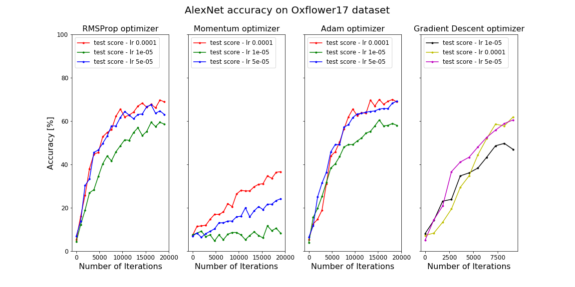
3.3 AlexNet Performance
As a comparison, have a look at the LeNet5 CNN performance on the larger oxflower17 dataset:
4. Final Words
The code is also available in my GitHub repository, so feel free to use it on your own dataset(s).
There is much more to explore in the world of Deep Learning; Recurrent Neural Networks, Region-Based CNN’s, GAN’s, Reinforcement Learning, etc. In future blog-posts I’ll build these types of Neural Networks, and also build awesome applications with what we have already learned. So subscribe and stay tuned!
[1] If you feel like you need to refresh your understanding of CNN’s, here are some good starting points to get you up to speed:
- Machine Learning is fun!
- An Intuitive Explanation of Convolutional Neural Networks :
- CS231n Convolutional Neural Networks for Visual Recognition :
- Udacity’s Deep Learning course:
- Neural Networks and Deep Learning Ch 6. [2] If you want more information about the theory behind these different Neural Networks, Adit Deshpande’s blog post provides a good comparison of them with links to the original papers. Eugenio Culurciello has a nice blog and article worth a read. In addition to that, also have a look at this github repository containing awesome deep learning papers, and this github repository where deep learning papers are ordered by task and date.
