
The Python code for Logistic Regression can be forked/cloned from my Git repository. It is also available on PyPi. The relevant information in the blog-posts about Linear and Logistic Regression are also available as a Jupyter Notebook on my Git repository.
Introduction
In the previous blog we have seen the theory and mathematics behind the Logistic Regression Classifier. Logistic Regression is one of the most powerful classification methods within machine learning and can be used for a wide variety of tasks. Think of pre-policing or predictive analytics in health; it can be used to aid tuberculosis patients, aid breast cancer diagnosis, etc. Think of modeling urban growth, analysing mortgage pre-payments and defaults, forecasting the direction and strength of stock market movement, and even sports.
Reading all of this, the theory[1]of Logistic Regression Classification might look difficult. In my experience, the average Developer does not believe they can design a proper Logistic Regression Classifier from scratch. I strongly disagree: not only is the mathematics behind is relatively simple, it can also be implemented with a few lines of code.
I have done this in the past month, so I thought I’d show you how to do it. The code is in Python but it should be relatively easy to translate it to other languages. Some of the examples contain self-generated data, while other examples contain real-world (iris) data. As was also done in the blog-posts about the bag-of-words model and the Naive Bayes Classifier, we will also try to automatically classify the sentiments of Amazon.com book reviews.
Short recap of the theory
We have seen that the technique to perform Logistic Regression is similar to regular Regression Analysis. There is a function \(h( \theta )\) which maps the input values \(X\) to the output \(Y\) and this function is completely determined by its parameters \(\theta\). So once we have determined the \(\theta\) values with training examples, we can determine the class of any new example.
We are trying to estimate the feature values \(\theta\) with the iterative Gradient Descent method. In the Gradient Descent method, the values of the parameters \(\theta\) in the current iteration are calculated by updating the values of \(\theta\) from the previous iteration with the gradient of the cost function \(J\).
In (regular) Regression this hypothesis function can be any function which you expect will provide a good model of the dataset. In Logistic Regression the hypothesis function is always given by the Logistic function:
\(h_{\theta} = \frac{1}{1 + \exp(-z)}} = \frac{1}{1 + \exp(-\theta x)}\).
Different cost functions exist, but most often the log-likelihood function known as binary cross-entropy (see equation 2 of previous post) is used.
One of its benefits is that the gradient of this cost function, turns out to be quiet simple, and since it is the gradient we use to update the values of \(\theta\) this makes our work easier.
Taking all of this into account, this is how Gradient Descent works:
- Make an initial but intelligent guess for the values of the parameters \(\theta\).
- Keep iterating while the value of the cost function has not met your criteria*:
- With the current values of \(\theta\), calculate the gradient of the cost function \(J\) ( \(\Delta \theta = - \alpa \frac{d}{d\theta} J(x)\) ).
- Update the values for the parameters \(\theta := \theta + \alpha \Delta \theta\)
- Fill in these new values in the hypothesis function and calculate again the value of the cost function;
*Usually the iteration stops when either the maximum number of iterations has been reached, or the error (the difference between the cost of this iteration and the cost of the previous iteration) is smaller than some minimum error value (0.001).
Regression Analysis
We have seen the self-generated example of students participating in a Machine Learning course, where their final grade depended on how many hours they had studied.
First, let’s generate the data:
1
2
3
4
5
6
7
8
9
10
11
12
13
14
15
16
17
18
19
20
21
22
23
import random
import numpy as np

num_of_datapoints = 100
x_max = 10
initial_theta = [1, 0.07]

def func1(X, theta, add_noise = True):
    if add_noise:
        return theta[0]*X[0] + theta[1]*X[1]**2 + 0.25*X[1]*(random.random()-1)
    else:
        return theta[0]*X[0] + theta[1]*X[1]**2

def generate_data(num_of_datapoints, x_max, theta):
    X = np.zeros(shape=(num_of_datapoints, 2))
    Y = np.zeros(shape=num_of_datapoints)
    for ii in range(num_of_datapoints):
        X[ii][0] = 1
        X[ii][1] = (x_max*ii) / float(num_of_datapoints)
        Y[ii] = func1(X[ii], theta)
    return X, Y

X, Y = generate_data(num_of_datapoints, x_max, initial_theta)
We can see that we have generated 100 points uniformly distributed over the \(x\)-axis. For each of these \(x\) - points the \(y\)-value is determined by \(y = 1 + 0.07 x^{2}\) minus some random value.
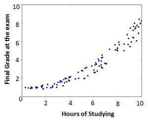
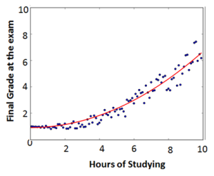
On the left we can see a scatterplot of the datapoints and on the right we can see the same data with a curve fitted through the points. This is the curve we are trying to estimate with the Gradient Descent method. This is done as follows:
1
2
3
4
5
6
7
8
9
10
11
12
13
14
15
16
17
numIterations= 1000
alpha = 0.00000005
m, n = np.shape(X)
theta = np.ones(n)

theta = gradient_descent(X, Y, theta, alpha, m, numIterations)

def gradient_descent(X, Y, theta, alpha, m, number_of_iterations):
    for ii in range(0,number_of_iterations):
        print "iteration %s : feature-value: %s" % (ii, theta)
        hypothesis = np.dot(X, theta)
        cost = sum([theta[0]*X[iter][0]+theta[1]*X[iter][1]-Y[iter] for iter in range(m)])
        grad0 = (2.0/m)*sum([(func1(X[iter], theta, False) - Y[iter])*X[iter][0]**2 for iter in range(m)])
        grad1 = (2.0/m)*sum([(func1(X[iter], theta, False) - Y[iter])*X[iter][1]**4 for iter in range(m)])
        theta[0] = theta[0] - alpha * grad0
        theta[1] = theta[1] - alpha * grad1
    return theta
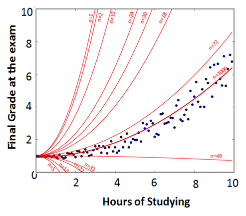
We can see that we have to calculate the gradient of the cost function \(n\) times and update the \(n\) feature values simultaneously! This indeed results in the curve we were looking for:
1
2
3
4
5
6
7
8
9
10
11
12
13
14
15
16
17
18
iteration 0 : feature-value: [ 1. 1.]
iteration 1 : feature-value: [ 0.99999688  0.98697306]
iteration 2 : feature-value: [ 0.99999381  0.97412576]
iteration 3 : feature-value: [ 0.99999078  0.96145564]
iteration 4 : feature-value: [ 0.99998779  0.94896025]
iteration 5 : feature-value: [ 0.99998485  0.93663719]
iteration 6 : feature-value: [ 0.99998194  0.92448406]
iteration 7 : feature-value: [ 0.99997907  0.91249854]
iteration 8 : feature-value: [ 0.99997624  0.90067831]
iteration 9 : feature-value: [ 0.99997345  0.88902108]
iteration 10 : feature-value: [ 0.9999707   0.87752462]
iteration 11 : feature-value: [ 0.99996799  0.86618671]
iteration 12 : feature-value: [ 0.99996531  0.85500515]
iteration 13 : feature-value: [ 0.99996268  0.84397779]
iteration 14 : feature-value: [ 0.99996007  0.83310251]
iteration 15 : feature-value: [ 0.99995751  0.82237721]
...
...
Logistic Regression
After this short example of Regression, lets have a look at a few examples of Logistic Regression. We will start out with a the self-generated example of students passing a course or not and then we will look at real world data.
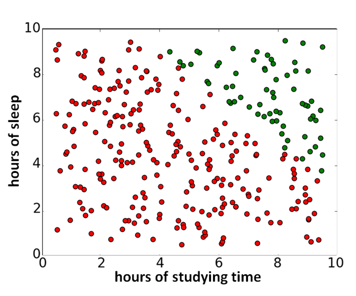
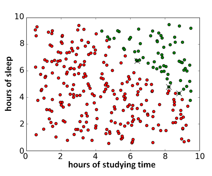
Let’s generate some data points. There are \(n = 300\) students participating in the course Machine Learning and whether a student \(i\) passes ( \(y_i = 1\)) or not ( \(y_i = 0\) ) depends on two variables;
- \(x_i^{(1)}\) : how many hours student \(i\) has studied for the exam.
- \(x_i^{(2)}\) : how many hours student \(i\) has slept the day before the exam.
1
2
3
4
5
6
7
8
9
10
11
12
13
14
15
16
17
18
19
20
21
22
23
24
import random
import numpy as np

def func2(x_i):
    if x_i[1] <= 4:
        y = 0
    else:
        if x_i[1]+x_i[2] <= 13:
            y = 0
        else:
            y = 1
    return y

def generate_data2(no_points):
    X = np.zeros(shape=(no_points, 3))
    Y = np.zeros(shape=no_points)
    for ii in range(no_points):
        X[ii][0] = 1
        X[ii][1] = random.random()*9+0.5
        X[ii][2] = random.random()*9+0.5
        Y[ii] = func2(X[ii])
    return X, Y

X, Y = generate_data2(300)
In our example, the results are pretty binary; everyone who has studied less than 4 hours fails the course, as well as everyone whose studying time + sleeping time is less than or equal to 13 hours (\(x_i^{(1)} + x_i^{(2)} \leq 13\)). The results looks like this (the green dots indicate a pass and the red dots a fail):
 ]
]
We have a LogisticRegression class, which sets the values of the learning rate \(\alpha\) and the maximum number of iterations at its initialization. The values of X, Y are set when these matrices are passed to the “train()” function, and then the values of no_examples, no_features, and theta are determined.
1
2
3
4
5
6
7
8
9
10
11
12
13
14
15
16
17
18
import numpy as np

class LogisticRegression():
    """
    Class for performing logistic regression.
    """
    def __init__(self, learning_rate = 0.7, max_iter = 1000):
        self.learning_rate = learning_rate
        self.max_iter = max_iter
        self.theta = []
        self.no_examples = 0
        self.no_features = 0
        self.X = None
        self.Y = None

    def add_bias_col(self, X):
        bias_col = np.ones((X.shape[0], 1))
        return np.concatenate([bias_col, X], axis=1)
We also have the hypothesis, cost and gradient functions:
1
2
3
4
5
6
7
8
9
10
11
12
13
14
15
def hypothesis(self, X):
    return 1 / (1 + np.exp(-1.0 * np.dot(X, self.theta)))

def cost_function(self):
    """
    We will use the binary cross entropy as the cost function. https://en.wikipedia.org/wiki/Cross_entropy
    """
    predicted_Y_values = self.hypothesis(self.X)
    cost = (-1.0/self.no_examples) * np.sum(self.Y * np.log(predicted_Y_values) + (1 - self.Y) * (np.log(1-predicted_Y_values)))
    return cost

def gradient(self):
    predicted_Y_values = self.hypothesis(self.X)
    grad = (-1.0/self.no_examples) * np.dot((self.Y-predicted_Y_values), self.X)
    return grad
With these functions, the gradient descent method can be defined as:
1
2
3
4
5
6
def gradient_descent(self):
    for iter in range(1,self.max_iter):
        cost = self.cost_function()
        delta = self.gradient()
        self.theta = self.theta - self.learning_rate * delta
        print("iteration %s : cost %s " % (iter, cost))
These functions are used by the “train()” method, which first sets the values of the matrices X, Y and theta, and then calls the gradient_descent method:
1
2
3
4
5
6
def train(self, X, Y):
    self.X = self.add_bias_col(X)
    self.Y = Y
    self.no_examples, self.no_features = np.shape(X)
    self.theta = np.ones(self.no_features + 1)
    self.gradient_descent()
Once the \(\theta\) values have been determined with the gradient descent method, we can use it to classify new examples:
1
2
3
4
5
def classify(self, X):
    X = self.add_bias_col(X)
    predicted_Y = self.hypothesis(X)
    predicted_Y_binary = np.round(predicted_Y)
    return predicted_Y_binary
Using this algorithm for gradient descent, we can correctly classify 297 out of 300 datapoints of our self-generated example (wrongly classified points are indicated with a cross).
Logistic Regression on the Iris Dataset
Now that the concept of Logistic Regression is a bit more clear, let’s classify real-world data! One of the most famous classification datasets is The Iris Flower Dataset. This dataset consists of three classes, where each example has four numerical features.
1
2
3
4
5
6
7
8
9
10
11
12
13
14
15
16
17
18
19
20
21
22
23
24
25
26
27
import pandas as pd

to_bin_y = { 1: { 'Iris-setosa': 1, 'Iris-versicolor': 0, 'Iris-virginica': 0 },
             2: { 'Iris-setosa': 0, 'Iris-versicolor': 1, 'Iris-virginica': 0 },
             3: { 'Iris-setosa': 0, 'Iris-versicolor': 0, 'Iris-virginica': 1 }
             }

#loading the dataset
datafile = '../datasets/iris/iris.data'
df = pd.read_csv(datafile, header=None)
df_train = df.sample(frac=0.7)
df_test = df.loc[~df.index.isin(df_train.index)]
X_train = df_train.values[:,0:4].astype(float)
y_train = df_train.values[:,4]
X_test = df_test.values[:,0:4].astype(float)
y_test = df_test.values[:,4]

Y_train = np.array([to_bin_y[3][x] for x in y_train])
Y_test = np.array([to_bin_y[3][x] for x in y_test])

print("training Logistic Regression Classifier")
lr = LogisticRegression()
lr.train(X_train, Y_train)
print("trained")
predicted_Y_test = lr.classify(X_test)
f1 = f1_score(predicted_Y_test, Y_test, 1)
print("F1-score on the test-set for class %s is: %s" % (1, f1))
As you can see, our simple LogisticRegression class can classify the iris dataset with quiet a high accuracy:
1
2
3
4
5
6
7
8
9
10
11
12
13
training Logistic Regression Classifier
iteration 1 : cost 8.4609605194
iteration 2 : cost 3.50586831057
iteration 3 : cost 3.78903735339
iteration 4 : cost 6.01488933456
iteration 5 : cost 0.458208317153
iteration 6 : cost 2.67703502395
iteration 7 : cost 3.66033580721
(...)
iteration 998 : cost 0.0362384208231
iteration 999 : cost 0.0362289106001
trained
F1-score on the test-set for class 1 is: 0.973225806452
For a full overview of the code, please have a look at GitHub.
Maximum Entropy Text Classification
Logistic Regression by using Gradient Descent can also be used for NLP / Text Analysis tasks. There are a wide variety of tasks which can are done in the field of NLP; autorship attribution, spam filtering, topic classification and sentiment analysis.
For a task like sentiment analysis we can follow the same procedure. We will have as the input a large collection of labelled text documents. These will be used to train the Logistic Regression classifier. The most important task then, is to select the proper features which will lead to the best sentiment classification. Almost everything in the text document can be used as a feature[2]; you are only limited by your creativity.
For sentiment analysis usually the occurence of (specific) words is used, or the relative occurence of words (the word occurences divided by the total number of words).
As we have done before, we have to fill in the \(X\) and \(Y\) matrices, which will serve as an input for the gradient descent algorithm and this algorithm will give us the resulting feature vector \(\theta\). With this vector we can determine the class of other text documents.
As always \(Y\) is a vector with \(n\) elements (where \(n\) is the number of text-documents). The matrix \(X\) is a \(n\) by \(m\) matrix; here \(m\) is the total number of relevant words in all of the text-documents. I will illustrate how to build up this \(X\) matrix with three book reviews:
- pos: “This is such a beautiful edition of Harry Potter and the Sorcerer’s Stone. I’m so glad I bought it as a keep sake. The illustrations are just stunning.” (28 words in total)
- pos: “A brilliant book that helps you to open up your mind as wide as the sky” (16 words in total)
- neg: “This publication is virtually unreadable. It doesn’t do this classic justice. Multiple typos, no illustrations, and the most wonky footnotes conceivable. Spend a dollar more and get a decent edition.” (30 words in total)
These three reviews will result in the following \(X\)-matrix.
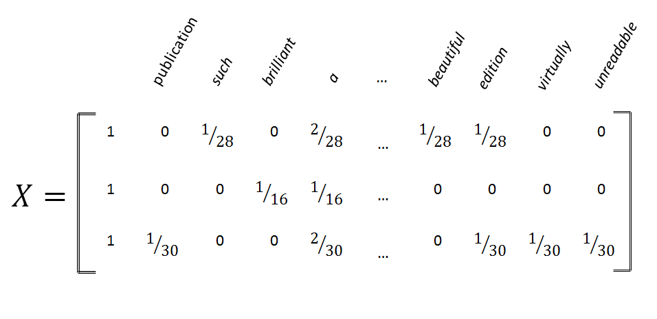
As you can see, each row of the \(X\) matrix contains all of the data per review and each column contains the data per word. If a review does not contain a specific word, the corresponding column will contain a zero. Such a \(X\)-matrix containing all the data from the training set can be build up in the following manner:
Assuming that we have a list containing the data from the training set:
1
2
3
4
5
6
[
([u'downloaded', u'the', u'book', u'to', u'my', ..., u'art'], 'neg'),
([u'this', u'novel', u'if', u'bunch', u'of', ..., u'ladies'], 'neg'),
([u'forget', u'reading', u'the', u'book', u'and', ..., u'hilarious!'], 'neg'),
...
]
From this training_set, we are going to generate a words_vector. This words_vector is used to keep track to which column a specific word belongs to. After this words_vector has been generated, the \(X\) matrix and \(Y\) vector can filled in.
1
2
3
4
5
6
7
8
9
10
11
12
13
14
15
16
17
18
19
20
21
22
23
24
25
26
27
28
29
30
31
32
def generate_words_vector(training_set):
    words_vector = []
    for review in training_set:
        for word in review[0]:
            if word not in words_vector: words_vector.append(word)
    return words_vector

def generate_Y_vector(training_set, training_class):
    no_reviews = len(training_set)
    Y = np.zeros(shape=no_reviews)
    for ii in range(0,no_reviews):
        review_class = training_set[ii][1]
        Y[ii] = 1 if review_class == training_class else 0
    return Y

def generate_X_matrix(training_set, words_vector):
    no_reviews = len(training_set)
    no_words = len(words_vector)
    X = np.zeros(shape=(no_reviews, no_words+1))
    for ii in range(0,no_reviews):
        X[ii][0] = 1
        review_text = training_set[ii][0]
        total_words_in_review = len(review_text)
        for word in Set(review_text):
            word_occurences = review_text.count(word)
            word_index = words_vector.index(word)+1
            X[ii][word_index] = word_occurences / float(total_words_in_review)
    return X

words_vector = generate_words_vector(training_set)
X = generate_X_matrix(training_set, words_vector)
Y_neg = generate_Y_vector(training_set, 'neg')
As we have done before, the gradient descent method can be applied to derive the feature vector from the \(X\) and \(Y\) matrices:
1
2
3
4
5
numIterations = 100
alpha = 0.55
m,n = np.shape(X)
theta = np.ones(n)
theta_neg = gradient_descent2(X, Y_neg, theta, alpha, m, numIterations)
What should we do if a specific review tests positive (Y=1) for more than one class? A review could result in Y=1 for both the neu class as well as the neg class. In that case we will pick the class with the highest score. This is called multinomial logistic regression.
Maximum Entropy Text Classification with Python’s NLTK library
So far, we have seen how to implement a Logistic Regression Classifier in its most basic form. It is true that building such a classifier from scratch, is great for learning purposes. It is also true that no one will get to the point of using deeper / more advanced Machine Learning skills without learning the basics first.
For real-world applications however, often the best solution is to not re-invent the wheel but to re-use tools which are already available. Tools which have been tested thorougly and have been used by plenty of smart programmers before you. One of such a tool is Python’s NLTK library.
NLTK is Python’s Natural Language Toolkit and it can be used for a wide variety of Text Processing and Analytics jobs like tokenization, part-of-speech tagging and classification. It is easy to use and even includes a lot of text corpora, which can be used to train your model if you have no training set available.
Let us also have a look at how to perform sentiment analysis and text classification with NLTK. As always, we will use a training set to train NLTK’s Maximum Entropy Classifier and a test set to verify the results. Our training set has the following format:
1
2
3
4
5
6
training_set = [
([u'this', u'novel', u'if', u'bunch', u'of', u'childish', ..., u'ladies'], 'neg')

([u'where', u'to', u'begin', u'jeez', u'gasping', u'blushing', ...,  u'fail????'], 'neg')
...
]
As you can see, the training set consists of a list of tuples of two elements. The first element is a list of the words in the text of the document and the second element is the class-label of this specific review (‘neg’, ‘neu’ or ‘pos’). Unfortunately NLTK’s Classifiers only accepts the text in a hashable format (dictionaries for example) and that is why we need to convert this list of words into a dictionary of words.
1
2
3
4
def list_to_dict(words_list):
  return dict([(word, True) for word in words_list])

training_set_formatted = [(list_to_dict(element[0]), element[1]) for element in training_set]
Once the training set has been converted into the proper format, it can be feed into the train method of the MaxEnt Classifier:
1
2
3
4
5
6
7
import nltk

numIterations = 100

algorithm = nltk.classify.MaxentClassifier.ALGORITHMS[0]
classifier = nltk.MaxentClassifier.train(training_set_formatted, algorithm, max_iter=numIterations)
classifier.show_most_informative_features(10)
Once the training of the MaxEntClassifier is done, it can be used to classify the review in the test set:
1
2
3
4
5
for review in test_set_formatted:
    label = review[1]
    text = review[0]
    determined_label = classifier.classify(text)
    print determined_label, label
Final Words:
So far we have seen the theory behind the Naive Bayes Classifier and how to implement it (in the context of Text Classification) and in the previous and this blog-post we have seen the theory and implementation of Logistic Regression Classifiers. Although this is done at a basic level, it should give some understanding of the Logistic Regression method (I hope at a level where you can apply it and classify data yourself). There are however still many (advanced) topics which have not been discussed here:
- Which hill-climbing / gradient descent algorithm to use; IIS (Improved Iterative Scaling), GIS (Generalized Iterative Scaling), BFGS, L-BFGS or Coordinate Descent
- Encoding of the feature vector and the use of dummy variables
- Logistic Regression is an inherently sequential algorithm; although it is quiet fast, you might need a parallelization strategy if you start using larger datasets.
If you see any errors please do not hesitate to contact me. If you have enjoyed reading, maybe even learned something, do not forget to subscribe to this blog and share it!
[1] See the paper of Nigam et. al. on Maximum Entropy and the paper of Bo Pang et. al. on Sentiment Analysis using Maximum Entropy. Also see Using Maximum Entropy for text classification (1999), A simple introduction to Maximum Entropy models(1997), A brief MaxEnt tutorial, and another good MIT article.
[2] See for example Chapter 7 of Speech and Language Processing by (Jurafsky & Martin): For the task of period disambiguation a feature could be whether or not a period is followed by a capital letter unless the previous word is St.