In this blog-post we will have a look at how Differential Equations (DE) can be solved numerically via the Finite Differences method. By solving differential equations we can run simulations of dynamical systems and make predictions about the world.
The reason for writing this blog-post is because I am interested in a new type of Neural Networks called Physics Informed Neural Networks (PINN). This is an emerging field where traditional scientific computing and modern machine learning are converging. It is also known under several other names like Scientific Machine Learning or Physics Based Deep Learning. We will talk about it in more detail in a later blog-post, but it basically consists of solving differential equations with Neural Networks. The idea behind is, is that since Neural Networks are universal function approximators they can be used for solving any function. So with a small adaptation to the loss function they can also be used to solve differential equations describing the laws of nature. This field is still in its infancy, but already some significant results have been demonstrated.
But before we can understand how these PINNs work and how DE’s can be solved with Neural Networks, we first have to understand how differential equations are solved traditionally via scientific computing methods. That is why in this blog-post we will go into what Differential Equations are, and how they can be solved numerically with the Finite Differences method.
Why should you read this blog-post? The First reason is if you want to understand what Differential Equations approximately are, what they are used for and how you can model them numerically. Even if you will never use it in your professional live I think it a good idea to know the bare minimum about this topic.
For most people Differential Equations are a strange and distant topic they may have followed a course about, but never have used it afterwards. Since nobody likes too much theory, we will keep the mathematical equations to a minimum and explain as much as possible with illustrations and Python code. No mathematics just for the sake of mathematics!
1. An Introduction to Differential Equations
What are differential equations exactly? In order to understand that we first need to understand what regular equations and functions are. So let’s go into some definitions regarding this.
Univariate vs Multivariate Equations
Equations can be divided into into univariate and multivariate equations.
The difference between univariate and multivariate is that with univariate the function describing the system depends on only one variable f = f(x) while for multivariate systems the function depends on more than one variable \(f = f(x, y, z, ..)\) or \(f = f(x_1, x_2, x_3, ...)\). Univariate functions are usually easier to solve but more boring since you can only use it to describe very simple systems.
Linear vs Non-Linear functions
Also a distinction can be made between linear and non-linear problems.
A linear function satisfies the superposition principle. That means that it satisfies the following two conditions:
- additivity: \(f(x + y) = f(x) + f(y)\) and,
- homogeneity: \(f(a \cdot x) = a \cdot f(x)\). A nonlinear function is a function that does not satisfy the superposition principle.
1.2 Fitting a linear equation to data
Let’s say that we have a dataset of with n numerical values (columns) and m rows and we are trying to find an equation which accurately describes this dataset. This process of finding the equation is also known as regression.
Below we can see the Energy efficiency dataset, which contains eight variables used to estimate the heating load of buildings.
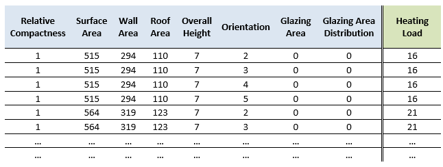 Figure 1. The Energy Efficiency dataset.
Each line (row) in the dataset can be seen as a linear equation, i.e.
\[a_1 x_1 + a_2 x_2 + a_3 x_3 + a_4 x_4 + a_5 x_5 + a_6 x_6 + a_5 x_5 + a_6 x_6 = y\]and the entire dataset can be seen as a system of linear equations.
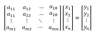 Figure 2. A system of linear equations.
The function which best describes this system of linear equations can be found using well known techniques in Linear Algebra.
A direct approach is to compute the inverse of matrix A and multiply it with the y-vector, i.e. \(x = A^{-1} \cdot y\) We can also use LU-decomposition instead of calculating the inverse of A. Or a better approach is to use the iterative Gradient Descent method since it is computationally less expensive. Also see previous blog post. Of course the models get more complicated when we have more complex data. If our dataset consists of a lot of images, we might need to use layers and layers of these linear equations in combination with convolutional filters (see Convolutional Neural Networks) and if our dataset consists of time-series data we might need to use (stochastic) signal analysis techniques in order to convert these time-series data (of variable length) into features.
1.3 What is the difference between a regular equation and a differential equation?
We have seen that a regular equation is a function y that can be expressed in one or more variables;
\(f = f(x_1, x_2, .., x_n)\) .
The difference between an equation and a differential equation is that a differential equation does not only contain the function and the variables of the function, but also the derivatives of the function with respect (one of) the variables
\(f = f(x_1, x_2, .., x_n, \frac{dy}{dx_i})\) .
As you might know, the derivative of a function gives the rate-of-change of that function.
A regular equation describes how a function changes with respect to its variables. So it tells us what happens to the value of y when we change the value of \(x_1\) and what happens if we change the value of \(x_2\). Since a differential equation also contains derivatives, we do not only know what happens to y if we change the value of \(x_1\) and \(x_2\), but also what happens if we change the value of x_1 over time.
Since differential equations contain rate-of-changes (derivatives), they are ideal for describing dynamical systems. A dynamical system is a system whose state changes over time due to one of the variables of the system. If we want to know how a dynamical system change(s) over time, and how we can predict the future values from the past, we have to solve a differential equation.
Since many things in the real world are dynamical in nature, differential equations are used everywhere. Many problems can be reduced to differential equations, making them a very important part of Mathematics, Physics, Biology, Engineering and Economics. You can think of Newton’s law of motion, conservation of mass, transfer of heat, radioactive decay, Hooke’s law of elasticity, etc, etc.
1.3.1 Regular equations vs differential equations
So differential equations contain derivatives and describe dynamical systems while regular equations do not contain derivatives and describe static systems. It still sounds a little bit cryptic at this point. This description does not give a good understanding of what differential equations actually are. Another way to look at it is to consider a differential equation as an abstract generalization of regular equations.
To understand this, we have to remember that a regular equation is the abstract generalisation of functions (the inter-dependencies between variables). For example, below we have three functions describing three different processes;
- \(s(t) = 0.5*gt^2\) if the function for the distance covered by a falling object (where \(g = 9.81 m/s^2\) is the gravitational constant),
- \(E(v) = 0.5mv^2\) if the function for the kinetic energy of a falling object (where \(m\) is the mass of the object and \(v\) is the velocity),
- \(Q = 0.5 * RI^2\) is the function for the heat generated by a resistor.
All of these equations can be abstracted into the more general equation \(y = 0.5 * ax^2\) , where \(a\) is a constant which can take on the values of \(g\), \(m\) and \(R\). The now more abstract equation no longer depends on the concrete values of \(t\), \(v\), \(I\) but on \(x\). We can fill in these values for \(a\) and \(x\) go from the more abstract equation \(y = 0.5 * ax^2\) to a specific equation describing a specific process.
So if regular equations are generalized abstractions of specific functions, then differential equations are living one level higher and are generalized abstractions of regular equations. Just like a regular equation can describe a whole set of functions (by filling in concrete values into the equation), a differential equation can describe a whole set of regular equations. And by filling in the initial conditions we can go from a general form to a specific form.
In order to understand how a differential equation is a generalized abstraction of a regular equation, let us take an example of a regular equation and see how we can transform between this equation and its differential form.
The equation \(y = 2 - (x-3)^2\) describes a parabolic motion. We can go from this regular equation to its differential form by taking the derivative and then filling in the value of \(x\) as function of \(y\).
- \[y = 2 - (x-3)^2\]
- \[y - 2 = - (x - 3)^2\]
- \[2 - y = (x - 3)^2\]
- \[\sqrt{2-y} = x - 3\]
- \[x = (3 + \sqrt{2-y})\]
Above we have rewritten the equation such that \(x\) is a function of \(y\). If we take the derivative of \(y\) and then fill in the value of \(x\) we have gotten above, we can see how the differential form of this equation looks like:
- \[\frac{dy}{dx} = -2(x -3)\]
- \[\frac{dy}{dx} = -2 \sqrt{2-y}\]
Above we can see the differential form of our equation.
Now, lets solve this differential equation and see if we have done it correctly and what the regular equation(s) corresponding to this differential equation looks like. This can be done by techniques like separation of variables, integrating both sides and by substitution.
\(\frac{dy}{dx} = -2 \sqrt{2-y}\) \(\frac{1}{\sqrt{2-y}} dy = -2 dx\) \(\int \frac{1}{\sqrt{2-y}} dy = -2 \int dx\) \(-2 \sqrt{2-y} = -2x + c_1\) \(\sqrt{2-y} = x + c_2\) \(\sqrt{2-y} = x + c_2\) \(2-y = (x + c_2)^2\) \(y = 2 - (x + c_2)^2\)
As you can see, if we solve the differential equation, the solution is the equation \(y = 2 - (x-c_2)^2\) , where \(c_2\) is some constant.
This equation is equal to the equation we started with if we fill in the (initial) condition of \(c_2 = -3\) . As we can see, the differential equation describes our original equation, but since we can fill in infinitely many values for \(c_2\) it also describes infinitely many other equations.
We can get to the specific equation from the family of equations by filling in for the initial conditions.
1.3.2 Plotting Regular equations vs Differential Equations
In the previous section we have transformed a regular equation to its differential form and then transformed it back in order to understand how a differential equation describes a whole set of regular equations. This difference between regular and differential equations can also be understood visually, without using any mathematics.
Below we will plot a relatively simple differential equation. One which describes the mathematical pendulum; a mathematical pendulum is an idealized pendulum which can only move in a 2D plane and does not experience any air-resistance or gravity and hence does not slow down.
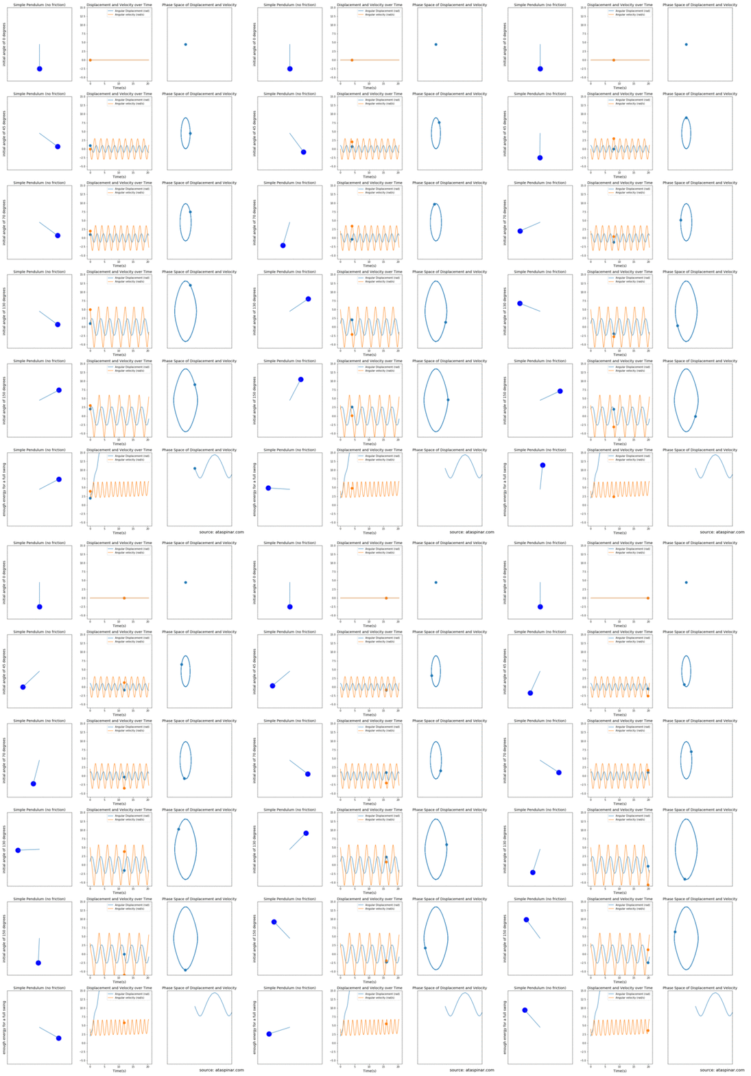 Figure 3. The mathematical pendulum (left figures) together with plots of the displacement and velocity over time (middle figures) and the phase-space of the displacement ánd velocity (right figures). This is done for several initial angles.
In Figure 3 we can see on the left most figures, the simple pendulum moving in the 2D plane, in the middle figures we can see the plots of the displacement and velocity over time and on the right most figures we can see a plot of the displacement vs the velocity. Depending on the starting angle, the pendulum will have a different displacement and velocity during the rest of its trajectory. Since the pendulum is idealized and does not experience any resistance, the maximum displacement and velocity values do not decay over time.
From top to bottom we see the different cases for when we start with an initial angle of:
- 0 degrees; the pendulum does not move at all and the displacement and velocity is also 0 over time. Since both the displacement and the velocity are zero, In the right most plot of velocity vs displacement this is a single point at (0,0).
- 45 degrees; Since there is no gravity or air-resistance the pendulum keeps moving between -45 and +45 degrees. At the top left and top right sides, the velocity becomes zero but the displacement is maximum and at the center the displacement is zero but the velocity is maximum. In the middle plot of velocity and displacement vs time we can see two sinusoidal plots shifted from each other by 90 degrees. In the right most plot, the velocity vs displacement plot becomes an ellipse.
- 70 / 130 and 150 degrees; here the pendulum behaves similar to one where the initial angle is 45 degrees. The main difference is that the maximum displacement and velocity values are larger and hence the ellipse in the right plots also becomes bigger.
- a full swing; If the pendulum has enough energy at the start for a full swing, it will keep on rotating in the same direction (since there is no resistance) and the displacement keeps increasing. The velocity does have a maximum and minimum value at the bottom and top of the swing. In the right most plot this becomes a sinusoid which keeps moving to the right (without an end).
In Figure 4 (below) we have plotted the different curves we have seen in the right figures of Figure 3 in a single figure. Such a figure is known as a phase-space plot. A phase-space plot gives all possible states a dynamical system can be in. Each point in a phase-space plot indicates one state and with arrows we can see how the system moves from one state to another. In Figure 4 we have indicated with the blue curves the trajectories in phase-space we also saw in Figure 3.
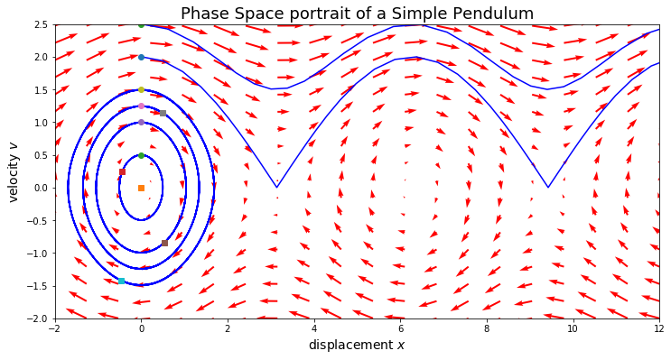 Figure 4. A plot of the phase-space of the simple pendulum. Depending on the initial conditions the curve will traverse the phase-space in a different way.
So to summarise, a differential equation describes a dynamical system and can be seen as an abstract generalisation of a normal equation. It has infinitely many solutions in its general form and we can go from a general solution to a particular solution by setting the values of the initial conditions. The phase-space describes all possible states of the dynamical system visually and shows us how a state evolves over time by tracing a path through this high-dimensional phase space.
1.4 Ordinary vs Partial Differential Equations
Another concept we should be aware of is that a differential equation can be Ordinary, or it can be Partial. An ordinary differential equation (ODE) only contains derivative(s) with respect to óne of its variables; if it contains a derivative w.r.t. \(x_1\) for example, it will not contain a derivative w.r.t. to the other variables \(x_2, x_3, ..., x_n\) .
A partial differential equation (PDE) has derivatives with respect to more than one of its variables, for example \(f = f(x_1, x_2, .., x_n, \frac{dy}{dx_1}, \frac{dy}{dx_2}, \frac{dy^2}{dx_1 x_2}, … )\) .
1.5 Splitting an higher order Differential Equation
Besides being Ordinary or Partial, differential equations are also specified by their order. The order of an differential equation indicates the largest derivative present in the equation. So if an ODE contains \(\frac{d^2y}{dx_i^2}\) it is a second order ODE.
Generally an ODE of a higher order is more difficult to solve, but the good thing is that an higher order ODE can always be rewritten as a system of coupled first order equations. This is done with the process of separation of variables.
For example, Newton’s equation of motion describe how a particle with mass m behaves when it experiences a Force \(F\):
\(m \frac{d^2 x}{dt^2} = F(x)\) .
This is a second order equation since it contains a second order derivative. But we can decompose it into two separate equations by defining the velocity \(v\) as the first derivative of \(x\).
\(\frac{dx}{dt} = v\) ,
\(\frac{dv}{dt} = \frac{1}{m}F(x)\) .
Both of the descriptions of Newtons equation of motion are equal.
If we have an ODE of the n-th order, it can be rewritten as a system of n ordinary equations, by introducing n new functions; \(y_1 = y, y_2 = \frac{dy}{dx}, …, y_n = \frac{d^{n-1}}{dx^{n-1}}\) .
This is illustrated in the figure below:
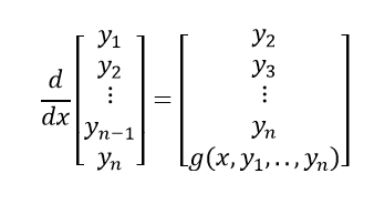 Figure 5. An ODE of order n, can be rewritten as a system of n ODE’s of order 1.
In the next section, we will see how we can solve differential equations numerically with the Finite Differences method.
2. How to solve a differential equation numerically
2.1 – The theory
There are several ways in which differential equations can be evaluated and solved numerically. There is the finite difference method (FDM), the finite volume method (FVM), the finite element method (FEM), or the spectral method.
All of them convert a continuous problem (differential equation) to a discrete problem so that it can be solved numerically. They differ in the way that they discretize the differential equation or the domain over which the differential equation has to be solved.
For example in the Finite Difference Method the domain is discretized by generating a square spatial-temporal grid with fixed size (and the differential equation is discretized with the finite difference operators). The Finite Element on the other hand does not discretize the domain in a grid of fixed size, but into a mesh of elements. These element can be shaped triangles or quadrangles in the 2D case, or tetrahedrons or hexahedrons in the 3D case. The Spectral method uses the Fourier transform to approximate the differential equation.
Here we will only focus on the Finite Difference Method since it is conceptually easier to understand and relatively easy to implement. The remainder of this section consists of a short description of how the Finite Difference method works, the different discretization schemes that can be used within FDM and we will end with a few examples in Python code.
Before we can solve a differential equation problem numerically we need to first discretize it in such a way it can be interpreted by a computer program. The discretization applies to two aspects; the differential equation itself needs to be discretized but also the domain over which the equation is going to be solved should be discretized.
- The discretization of the differential equation is done by transforming the mathematical operators to arithmetic operators which can operate on the grid points. The FD methods approximates derivates with finite difference operators using local Taylor expansions. The differential equation is written as a difference equation.
- The discretization of the domain is done by converting it to a structured grid of uniformly separated points. This can be a 1D, 2D or 3D grid of points. This is illustrated in the figure below.
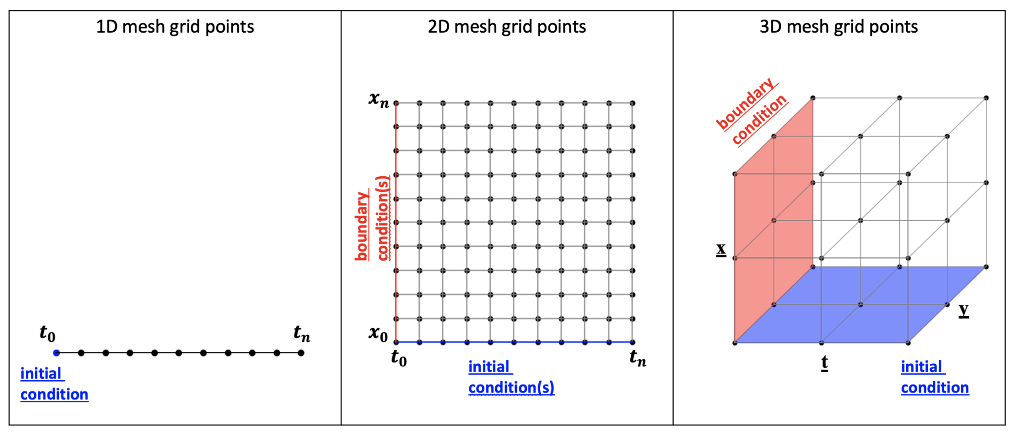 Figure 6. An illustration of the grid created for the finite difference method for solving differential equations in one (left), two (middle) and three (right) dimensions.
In the left most figure we can see the example of a grid in 1D space. We want to calculate the differential equation between \(t_0\) and \(t_n\) and have divided this domain into n equally spaced points. If we create a more finely spaced grid with more points, the approximation of the differential equation will be more accurate but it will take more time to finish the calculation. In this example we are looking at an equation which evolves over time \(t\) and hence we have a grid in time \(t_0, t_1, t_2, …, t_n\) . The value at the first point \(t_0\) is known and it is called the initial condition (or boundary condition in the case of a grid over \(x_0, x_1, x_2, …, x_n)\) .
In the middle figure we can see a grid in 2D space. The differential equation evolves over time and space and hence the grid is both in time \(t\) and in space \(x\).
In the right figure we have a grid in 3D space, with the grid of points defined in \(t\), \(x\) and \(y\).
Each point in the grids above is identified by one indices (\(i\)), two indices (\(i,j\)) in the case of the 2D grid or three indices (\(i, j, k\)) in the case of 3D grid. We don’t know what the value at the inner grid points are, but we know what the initial and/or boundary conditions are. Starting from the initial and/or boundary points we can calculate the values of the adjacent points. This is done with linear approximations.
In other words, we first calculate \(t_1\) from \(t_0\) (whose value is given by the initial condition), then \(t_2\) from \(t_1\), and continue this process until we have covered the entire domain.
This is how differential equations are solved numerically. As you can imagine, a differential equation can change quickly over time. The question then is how consistent, accurate and stable the numerical approximation of the differential equation is. Since we assume a linear variation between grid points, there will be some small error at each time step and over many time steps this can lead to a large global error.
One way to reduce the error is to reduce the size of the grid points; The smaller we make the stepsize, the smaller the truncation error becomes. However, every time you decrease the stepsize, the total number of points you have to calculate the solution over also increases. If you reduce the stepsize by a factor of two, the number of points increases by a factor of 2 in the 1D case, by a factor of 4 in the 2D case and by a factor of 9 in the 3D case.
Instead of reducing the stepsize, we can also change the discretization scheme used to approximate the slope between two adjacent points. We can choose a higher order discretization scheme. These higher order discretization schemes require more steps to calculate the values of adjacent points but have a much lower truncation error. In increasing order of complexity and accuracy, these discretization schemes consists of:
- First order solutions: Euler’s Methods: forward Euler, backward Euler, and semi-implicit Euler
- Second order solutions: Central Difference method, leapfrog method, and Heun’s Method (Second order Runge-Kutta)
- Higher order solutions: Runga-Kutta Methods (3rd order, 4th order Runge-Kutta)
Above we can see the different discretization schemes. The simplest way to approximate the slope between two adjacent points is the first order Euler’s method. There is the forward Euler and the backward Euler method. The difference between the forward Euler and Backward Euler methods is that for the forward Euler we take the forward difference and for the Backward Euler we take the backward difference. That means that for the forward Euler we use the value at \(t_n\) in order to calculate the value at \(t_{n+1}\), for the Backward Euler we use the value at \(t_n\) in order to calculate the value at \(t_{n-1}\). Euler’s method is a first order method, a simple and intuitive numerical method, but more error prone. The global error is proportional to \(\Delta t\).
We can also use Heun’s method, which is a second order method. Heun’s method uses a centered difference discretization scheme, i.e. it uses the average of the forward and the backward difference. Heun’s method has a global error proportional to \(\Delta t^2\).
So compared to the forward and backward Euler method, Heun’s method is much more accurate; if you make the time-step twice as small the error will be reduced by a factor of 2 with Euler’s method and by a factor of 4 with Heun’s method.
We saw that the first order method (Euler method) calculates one slope for one time step and has a global error proportional to \Delta t, the second order Heun’s method calculates (the average of) two slopes for one time step and has a global error proportional to \(\Delta t^2\). You can guess that the fourth order Runge-Kutta method will calculate (the average of) four different slopes for one time step in order to produce a slope estimation with a global error proportional to \(\Delta t^4\). An error proportional to \(\Delta t^4\) means that the error is reduced by a factor of 16 if you reduce step size by a factor of 2.
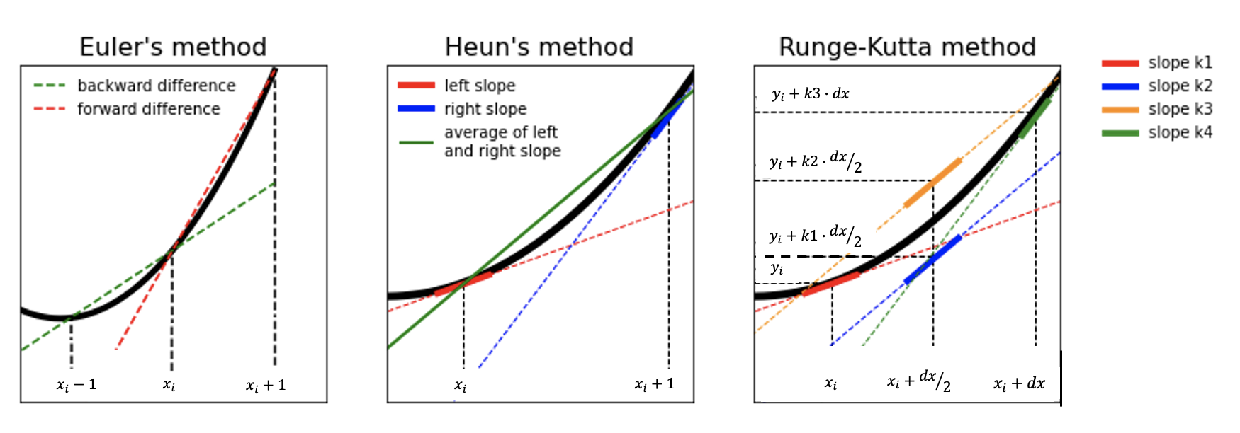 Figure 7. A schematic visualization of the several discretization schemes. In the left most figure we can see the Forward and Backward Euler methods, In the middle figure we can see the second order Heun’s method where two stages are used to estimate the slope, in the right figure we can see the fourth order Runge-Kutta method where four stages are used to estimate the slope.
Euler’s method, Heun’s Method and fourth order Runge-Kutta Method (RK4) are actually all part of the family of Runge-Kutte methods. Euler’s method is a first order RK method, and Heun’s method is a second order Runge-Kutta method (RK2). However, they are better known by their more popular names Euler’s method and Heun’s method. The fourth order Runge-Kutta is usually the one people refer to when they are talking about “Runge-Kutta”.
There are also fifth and sixth order Runge-Kutta methods, however the fourth order Runge-Kutta method is the most widely used one. Higher order RK methods only increase the accuracy incrementally while they do take more time to calculate, in other words; RK4 is good enough for most calculations.
As we have said before, the fourth order Runge-Kutta uses the weighted average of four slopes at four different locations.
- the first slope (called k1) is calculated at \(x_0\)
- the second slope (called k2) is calculated at a half step from \(x_0\) (that is at \(x_0 + dx/2\)) and it is calculated with the first slope k1.
- the third slope k3 is also calculated at a half step from \(x_0\), but the now known slope k2 is used instead of k1. Since k2 is the slope at half step \(x_0 + dx/2\) while k1 is the slope at \(x_0\) this will be a better approximation of the slope at a half step \(x_0 + dx/2\).
- the fourth slope k4 is calculated at a full step from \(x_0\) (at \(x_0 + dx\)) and the now known slope k3 is used to approximate the value at this location.
If you don’t understand all of the steps taken by the RK4 algorithm to calculate the average slope, don’t worry too much about it. The important thing to remember is that RK4 uses the weighted average of four slopes calculated at four different locations in order to estimate the slope between two points. If you still want to learn more about the derivation of RK4 you can have a look at this tutorial.
There are a lot of different discretization schemes which can be used when you solve a differential equation. When you have to choose between a lower order scheme or a higher order scheme, the trade-offs to consider are the following:
First order methods (like Euler’s method) are conceptually simple but inaccurate; they need smaller step sizes and more steps to achieve the same accuracy. Higher order methods (like RK4) are conceptually more complicated but accurate; they need less time steps to achieve the same accuracy, but each step requires more evaluations which also makes it slower.
You might think that you can simply just choose a simple scheme like Euler’s method as long as you keep the step size small enough and still achieve high accuracy. This is unfortunately not true. Besides the global error we have talked about (\(\Delta t^4\) for 4th order methods, \(\Delta t^2\) for 2nd order methods and \(\Delta t\) for 1st order methods), there is also a local error which is made at each step. When you keep decreasing the step sizes, after some point this local error starts to dominate over the global error, as beautifully explained here.
2.2 Solving Differential Equations numerically with Python
In the previous section we have seen the theory behind solving differential equations numerically. A quick summary of that section is that we need to:
- Discretize the differential equation such that it can operate on a grid of points, that is write the differential equation as a difference equation.
- Discretize the domain over which the differential equation has to be solved for, this will give us a structured grid of points, either in 1D, in 2D, in 3D or even higher dimensions.
- Choose one of the numerical methods for solving a difference equation, like the forward Euler method, Heun’s method, or RK4 method.
This looks and sounds simple enough, but how does it work in practice? The best way to understand it to look at some examples with Python code. In this section we will have a look several differential equations:
- (exponential) population growth; a first order differential equation which we will solve with the forward Euler method.
- 1D oscillating system; a second order differential equation which we will solve with the forward Euler method, Heun’s method and RK4.
2.2.1 population growth
One of the schoolbook examples of a first order ODE is population growth. This model can be applied to many systems like a population of bacteria cells, a population of animals, a population of humans, money in the bank, etc etc.
This can be given by the differential equation \(\frac{dN(t)}{dt} = r N(t)\). Here r is the growth rate of the population. The difference equation corresponding to this differential equation is:
\[\frac{dN(t)}{dt} = N(t+\Delta t) - N(t) = \Delta t r N(t)\]Lets see how this works in Python.
We can see that the function for calculating the Forward-Euler approximation of a differential equation has as input the initial conditions \(N_0\) (the initial population size), the growth rate r, the number of steps N_t. The step size dt is inverse proportional to the number of steps, \(dt = 8 / N_t\) .
1
2
3
4
5
6
7
8
def population_growth_FE(N_0, N_t, r, dt):
    N = np.zeros(N_t + 1)
    t = np.linspace(0, (N_t + 1)*dt, N_t + 1)
    N[0] = N_0
    # step forward in time
    for n in range(N_t):
        N[n+1] = N[n] + dt*r*N[n]
    return t, N
We start with two arrays t and N. The first one contains the time-axis and is filled in with linearly increasing values from \(t_0 = 0\) up to \(t_n\), each step is increasing with step size dt. The second array is empty and will be filled in by the forward Euler method.
Below we can see the solution for population growth with the initial condition \(N_0 = 100\) and the growth rate set to 0.5. In the first example we have set the number of steps to 20 and the stepwise to 0.4. The second example has 40 steps and the stepsize is 0.2.
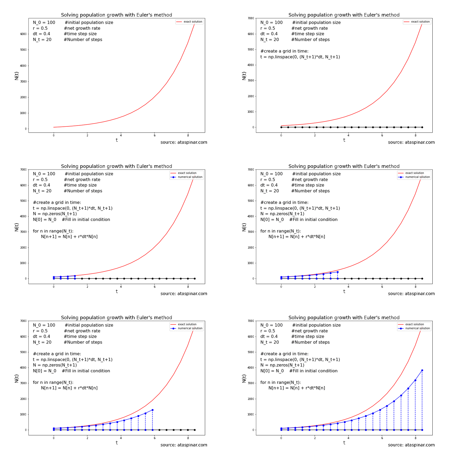 Figure 8. Solving population growth with the forward Euler method with 20 steps.
and
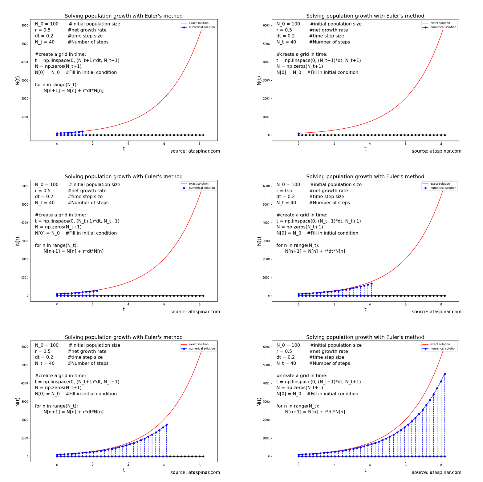 Figure 9. Solving population growth with the forward Euler method with 40 steps.
We can see that the accuracy of the solution strongly depends on the size of the time-step. So even though the Forward-Euler method is a simple method, its accuracy can be increased by decreasing the step-size and increasing the number of steps. As we have seen before, the step size can not be decreases indefinitely in order to achieve a high accuracy; at one point the local (truncation) error will starts to dominate over the global error. So at one point it makes more sense to switch to a higher order scheme like Heun’s method or RK4. This is what we will have a look at in the next example in section 2.2.2.
In this section we have looked at a model where the population grows exponentially with a rate \(r\). The population size only depended on the initial size \(N_0\) and the growth rate \(r\). This is not really realistic; in real life population growth is not described by an exponential function but by an logistic function. That is, population growth is S-shapes; at some point the population grow will decline due to a lack of resources, the presence of predators or other environmental factors.
If we want to make our model for population growth more realistic, we have to make the growth rate depend on the population size, so \(r = r(N)\).
This gives us the equation \(N^{n+1} = N^n + \Delta t \cdot r(N^n) \cdot N^n\)
To solve this equation, we need to calculate two values at each time-step. First we calculate the value of \(r(N)\) and then we can calculate the value of \(N^{n+1}\). This also means we have two equations to solve, one describing the growth rate as a function of \(N\) and one describing the population growth as a function of \(r\).
The Python code for this logistic model is:
1
2
3
4
5
6
7
8
9
10
11
12
13
def population_growth_logistic_FE(N_0, N_t, dt):
    # the growth rate function
    def growth_rate_r(N):
        return 0.1*(1-N/500)*N

    N = np.zeros(N_t + 1)
    t = np.linspace(0, N_t*dt, N_t+1)
    N[0] = N_0

    #step forward in time
    for n in range(N_t):
        N[n+1] = N[n] + dt*growth_rate_r(N[n])
    return t, N
In the next section we will have a look at the second order differential equation for a pendulum with gravity and friction.
2.2.2 Pendulum with gravity and friction
In this section we will have a look at a pendulum, but this time it does experience friction and gravity.
The second order differential equation describing this is given by:
\[\theta''(t) + b \cdot \theta(t) + c \cdot sin(\theta(t)) = 0\]where b and c are constants. As we can see, this is a second order differential equation. We can convert this to a system of first order differential equations by defining the angular velocity as the first derivative of the angular displacement.
\[\omega(t) = \theta'(t)\]With this we obtain the system of coupled first order differential equations:
\[\theta'(t) = \omega(t)\] \[\omega'(t) = -b \cdot \omega(t) - c \cdot sin(\theta(t))\]We will set the value of the constants b and c to 0.25 and 5.0 and have a look at the solution for \(\theta\) and \(\omega\) between \(t\) is 0 and 10.
1
2
3
4
5
6
7
8
9
10
from scipy.integrate import odeint

def damped_pendulum(y,t,b,c):
    theta, omega = y
    return np.array([omega, -b*omega - c*np.sin(theta)])

b, c = 0.25, 5.0
y0 = np.array([np.pi - 0.1, 0.0])
t = np.linspace(0,10,101)
exact_solution = odeint(damped_pendulum, y0, t, args=(b,c))
Here we have used scipy.integrate.odeint in order to get the exact solution of this differential equation.
If we plot how this looks like, we will get the following Figure:
1
2
3
4
5
6
7
8
9
10
11
12
13
14
fig, (ax0,ax1) = plt.subplots(figsize=(12,3),ncols=2)
ax0.plot(t, exact_solution[:, 0], 'k', label=r'exact', linewidth=3)
ax1.plot(t, exact_solution[:, 1], 'k', label=r'exact', linewidth=3)
title0 = r'exact solution for $$\theta(t)$$'
title1 = r'exact solution for $$\omega(t)$$'
ax0.set_title(title0)
ax1.set_title(title1)
ax0.legend(loc='best')
ax1.legend(loc='best')
ax0.grid()
ax1.grid()
ax0.set_xlabel('t')
ax1.set_xlabel('t')
plt.show()
 Figure 10. The exact solution for the damped pendulum.
Now that we know how the exact solution for the damped pendulum is supposed to look like, let us have a look at how the solution that we get with Euler’s method, Heun’s method and RK4 looks like. We will do this for different grid sizes by varying the number of steps in t from 10 steps, to 20 steps, to 100 steps, and to 1000 steps.
As we have said before, the forward Euler method uses the forward difference and calculates the value at y[i+1] using the value at y[i]. The Python code for the forward-Euler method is given by:
1
2
3
4
5
6
7
8
def euler_method(f, y0, t, args=()):
    n = len(t)
    y = np.zeros((n, len(y0)))
    y[0] = y0
    for i in range(n - 1):
        deltat = t[i+1] - t[i]
        y[i+1] = y[i] + deltat * f(y[i], t[i], *args)
    return y
def euler_method(f, y0, t, args=()): n = len(t) y = np.zeros((n, len(y0))) y[0] = y0 for i in range(n - 1): deltat = t[i+1] - t[i] y[i+1] = y[i] + deltat * f(y[i], t[i], *args) return y
Heun’s method uses two stages to calculate the slope between two points and hence it needs an intermediary calculation of \(y^*\) to calculate the value at the next time-step:
1
2
3
4
5
6
7
8
9
def huen_method(f, y0, t, args=()):
    n = len(t)
    y = np.zeros((n, len(y0)))
    y[0] = y0
    for i in range(n - 1):
        deltat = t[i+1] - t[i]
        y_star = y[i] + f(y[i], t[i], *args) * deltat / 2.
        y[i+1] = y[i] + deltat * f(y_star, t[i] + deltat / 2., *args)
    return y
And as we have seen before, Runge-Kutta method uses four stages to calculate the slope at four different positions and then uses the weighted average of these four slopes to calculate the slope between two points. Therefore it needs four intermediary calculations to calculate the value at the next time step. The code for the RK4 calculation is given by:
1
2
3
4
5
6
7
8
9
10
11
12
def runge_kutta4(f, y0, t, args=()):
    n = len(t)
    y = np.zeros((n, len(y0)))
    y[0] = y0
    for i in range(n - 1):
        h = t[i+1] - t[i]
        k1 = f(y[i], t[i], *args)
        k2 = f(y[i] + k1 * h / 2., t[i] + h / 2., *args)
        k3 = f(y[i] + k2 * h / 2., t[i] + h / 2., *args)
        k4 = f(y[i] + k3 * h, t[i] + h, *args)
        y[i+1] = y[i] + (h / 6.) * (k1 + 2*k2 + 2*k3 + k4)
    return y
Now that we know how the Python code for the forward-Euler scheme, Heun’s method and fourth order Runge-Kutta looks like, let us move forward and create the grid in time. We will do this for four different step sizes, one where the time-axis consists of 10 steps, one for 20 steps, one for 100 steps and one for 1000 steps.
1
2
3
4
t_10 = np.linspace(0, 10, 11)
t_20 = np.linspace(0, 10, 21)
t_100 = np.linspace(0, 10, 101)
t_1000 = np.linspace(0, 10, 1001)
How will the solution for \theta and \omega look like for these four different grids and for the three different discretization schemes? We expect that the solution decreases in accuracy (for all three schemes) as the number of steps becomes smaller, but that higher order discretization schemes are more accurate for lower number of steps.
In order to test this, we will loop through the four different time-axis and three different discretization schemes and plot the results in a single figure.
1
2
3
4
5
6
7
8
9
10
11
12
13
14
15
16
17
18
19
20
21
22
23
dict_methods = {"Euler": euler_method, "Heun":huen_method, "RK4":runge_kutta4}
list_timegrids = [t_1000, t_100, t_20,  t_10]

fig, axarr = plt.subplots(figsize=(12,12),ncols=2,nrows=4,sharex=True)
for row_no, t_ in enumerate(list_timegrids):
    axarr[row_no, 0].plot(t, exact_solution[:, 0], 'k', label=r'exact', linewidth=3)
    axarr[row_no, 1].plot(t, exact_solution[:, 1], 'k', label=r'exact', linewidth=3)
    for methodname, method in dict_methods.items():
        solution = method(damped_pendulum, y0, t_, args=(b, c))
        title0 = r'$$\theta(t)$$ with '+str(len(t_)-1)+' steps'
        title1 = r'$$\omega(t)$$ with '+str(len(t_)-1)+' steps'
        axarr[row_no, 0].plot(t_, solution[:, 0], label=methodname, linestyle='--')
        axarr[row_no, 1].plot(t_, solution[:, 1], label=methodname, linestyle='--')
        axarr[row_no, 0].set_title(title0)
        axarr[row_no, 1].set_title(title1)
        axarr[row_no,0].legend(loc='best')
        axarr[row_no,1].legend(loc='best')
        axarr[row_no,0].grid()
        axarr[row_no,1].grid()
        if row_no == 3:
            axarr[row_no,0].set_xlabel('t')
            axarr[row_no,1].set_xlabel('t')
plt.show()
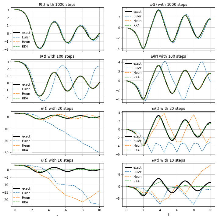 Figure 11.The numerical solution for theta and omega with the Euler method, Heun’s method and RK4, for four different time-axis.
As we can see, with 1000 steps in the time-axis all three methods give a pretty accurate solution, even though we can see Euler’s method start to deviate at larger values of t. For 100 steps, Heun’s method and RK4 are still accurate, but Euler’s method is already producing unreliable results. And as the number of steps in time becomes smaller, even Heun’s method becomes unreliable while RK4 still produces reliable results until the very end.
To see how large the difference in accuracy is for the three difference schemes, we vary the number of steps between 10 and 500 and plot the mean squared error as a function of the number of steps.
1
2
3
4
5
6
7
8
9
10
11
12
13
14
15
16
17
18
19
20
21
22
23
24
25
26
27
28
29
30
31
32
33
34
35
from sklearn.metrics import mean_squared_error
from collections import defaultdict

dict_error_theta = defaultdict(list)
dict_error_omega = defaultdict(list)
list_timesteps = range(11,502,10)

for nsteps in list_timesteps:
    t_ = np.linspace(0, 10, nsteps)
    for methodname, method in dict_methods.items():
        calculated_solution = method(damped_pendulum, y0, t_, args=(b, c))
        exact_solution = odeint(damped_pendulum, y0, t_, args=(b, c))
        calculated_theta = calculated_solution[:,0]
        calculated_omega = calculated_solution[:,1]
        exact_theta = exact_solution[:, 0]
        exact_omega = exact_solution[:, 1]
        mse_theta = mean_squared_error(exact_theta, calculated_theta)
        mse_omega = mean_squared_error(exact_omega, calculated_omega)
        dict_error_theta[methodname].append(mse_theta)
        dict_error_omega[methodname].append(mse_omega)

fig, (ax0, ax1) = plt.subplots(figsize=(10,4), ncols=2)
ax0.set_title(r'Error in calculation of $$\theta(t)$$', fontsize=15)
ax1.set_title(r'Error in calculation of $$\omega(t)$$', fontsize=15)
for k, v in dict_error_theta.items():
    ax0.plot(list_timesteps, v, label=f'{k}')
for k, v in dict_error_omega.items():
    ax1.plot(list_timesteps, v, label=f'{k}')
ax0.set_xlabel('number of time steps', fontsize=15)
ax1.set_xlabel('number of time steps', fontsize=15)
ax0.set_ylabel('mean squared error', fontsize=15)
ax1.set_ylabel('mean squared error', fontsize=15)
ax0.legend()
ax1.legend()
plt.show()
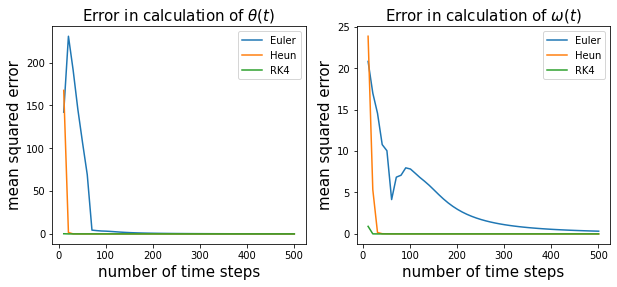 Figure 12.The mean square error for theta and omega for the forward-Euler, Heun’s method and RK4 as a function of the number of time-steps. As we can see RK4 and Heun’s method are already pretty accurate at very small number of time-steps while the forward Euler needs a much larger number of steps.
As we can see, the error in Heun’s method goes to zero fairly quickly. It doesn’t need more than 30 steps for an accurate calculation of \theta and not more than 40 steps for an accurate calculation of \(\omega\). For the RK4 method these number are even lower; 15 to 20 steps for an accurate calculation of \(\theta\) and \(\omega\). On the other hand Euler’s method needs at least 100 steps for an accurate calculation of \(\theta\) and 500+ steps for an accurate calculation of \(\omega\).
3. Final Thoughts and additional resources:
In this blog-post we have seen how we can solve differential equations numerically in Python. We have seen the Python code for the three most popular discretization schemes of first order, second order and fourth order: the forward-Euler method, Heun’s method and Runge-Kutta.
This should be sufficient as an introductionary post into differential equations and how we can solve them numerically. If you would like to know more about this topic, below is a good list of resources.
If you are interested in solving (Partial) Differential Equations in Python here are some resources I found very helpful:
- CFD Python is a module which teaches you how you can code basic partial differential equations that describe the physics of fluid flow. It is part of a course gives by Prof. Lorena Barba at Boston University and what I really like about this is that it builds up your CFD coding skills from scratch. There are 12 steps to coding the Navier-Stokes equation; you start with 1D linear convection, the 1D Burgers’ equation, 2D Burgers’ equation, Poisson equation in 2D and at step 12 you have to solve the Navier-Stokes equation for 2D channel flow.
- And then there are the videos of the CFD course.
- FEniCS tutorial, the GitHub repository corresponding to the book Solving PDEs in Python, The FEniCS Tutorial I. The book explains fundamental concepts of the finite element method, FEniCS programming, and has numerous examples of how to solve a range of PDEs. It is available as a free e-book.
- The same author also gives the course “numerical methods for partial differential equations” and the materials of this course are also available on its GitHub repository.
- The books of Solving Ordinary Differential Equations I and II from Hairer and Wanner
The should be enough as an introduction in Differential Equations and what the main difference is from regular equations. For people who are interested to learn more about this topic, I recommend V.I. Arnold’s book Ordinary Differential Equations which has an uniquely qualitative way of explaining differential equations and phase spaces.
There is also a wide range of software packages available in Python for solving ODE’s. These tools give you access to a lot of different solving methods, where most of them are more complicated / sophisticated then you could program by yourself (like adaptive step-size, ..).
These tools consist of SciPy, JITCode, PyDSTool, diffeqpy and ODESpy (unfortunately need Python 2.7). And of course you do not have to limit yourself to Python, since there nice ODE’s solving libraries available in almost all programming languages. You can have a look at this comparison between ODE Solver Suites in Julia, R, Matlab, Python, Fortran, C, Mathematica and Maple.
There are some other tools for solving PDE’s based on finite element method: sfepy, Fenics,