1. Introduction
In the previous blog post we have seen how to build Convolutional Neural Networks (CNN) in Tensorflow, by building various CNN architectures (like LeNet5, AlexNet, VGGNet-16) from scratch and training them on the MNIST, CIFAR-10 and Oxflower17 datasets.
It starts to get interesting when you start thinking about the practical applications of CNN and other Deep Learning methods. If you have been following the latest technical developments you probably know that CNNs are used for face recognition, object detection, analysis of medical images, automatic inspection in manufacturing processes, natural language processing tasks, any many other applications. You could say that you’re only limited by your imagination and creativity (and of course motivation, energy and time) to find practical applications for CNNs.
Inspired by Kaggle’s Satellite Imagery Feature Detection challenge, I would like to find out how easy it is to detect features (roads in this particular case) in satellite and aerial images.
If this is possible, the practical applications of it will be enormous. In a time of global urbanisation, cities are expanding, growing and changing continuously. This of course comes along with new infrastructures, new buildings and neighbourhoods and changing landscapes. Monitoring and keeping track of all of these changes has always been a really labour intensive job. If we could get fresh satellite images every day and use Deep Learning to immediately update all of our maps, it would a big help for everyone working in this field!
Developments in the field of Deep Learning are happening so fast that ‘simple’ image classification, which was a big hype a few years ago, already seems outdated. Nowadays, also object detection has become mainstream and in the next (few) years we will probably see more and more applications using image segmentation (see figure 1).
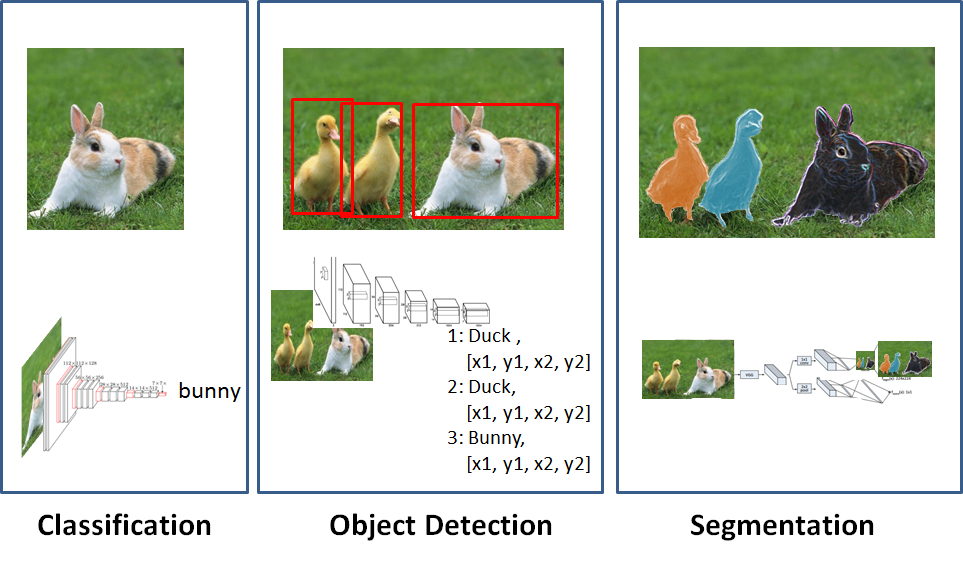 Figure 1: Tasks in Computer vision can be categorized as image classification, object detection or segmentation tasks.
In this blog we will use Image classification to detect roads in aerial images. To do this, we first need to get these aerial images, and get the data containing information on the location of roads (see Section 2.1). After that we need to map these two layers on top each other, we will do this in section 3.1. After saving the prepared dataset (Section 4.1) in the right format, we can feed it into our build convolutional neural network (Section 4.3). We will conclude this blog by looking at the accuracy of this method, and discuss which other methods can be used to improve it.
The code is now also available in a notebook on my GitHub repository
2 Getting the Data
The first (and often the most difficult) step in any Data Science project is always obtaining the data. Luckily there are many open datasets containing satellite images in various forms. There is the Landsat dataset, ESA’s Sentinel dataset, MODIS dataset, the NAIP dataset, etc. Each dataset has different pro’s and con’s. Some like the NAIP dataset offer a high resolution (one meter resolution), but only cover the US. Others like Landsat cover the entire earth but have a lower (30 meter) resolution. Some of them show which type of land-cover (forest, water, grassland) there is, others contain atmospheric and climate data.
Since I am from the Netherlands, I would like to use aerial / satellite images covering the Netherlands, so I will use the aerial images provided by PDOK. These are not only are quite up to date, but they also have an incredible resolution of 25 cm.
Dutch governmental organizations have a lot open-data available which could form the second layer on top of these aerial images. With Pdokviewer you can view a lot of these open datasets online;
- think of layers containing the infrastructure (various types of road, railways, waterways in the Netherlands (NWB wegenbestand),
- layers containing the boundaries of municipalities and districts,
- physical geographical regions,
- locations of every governmental organizations,
- agricultural areas,
- electricity usage per block,
- type of soil, geomorphological map,
- number of residents per block,
- surface usage, etc etc etc (even the living habitat of the brown long eared bat).
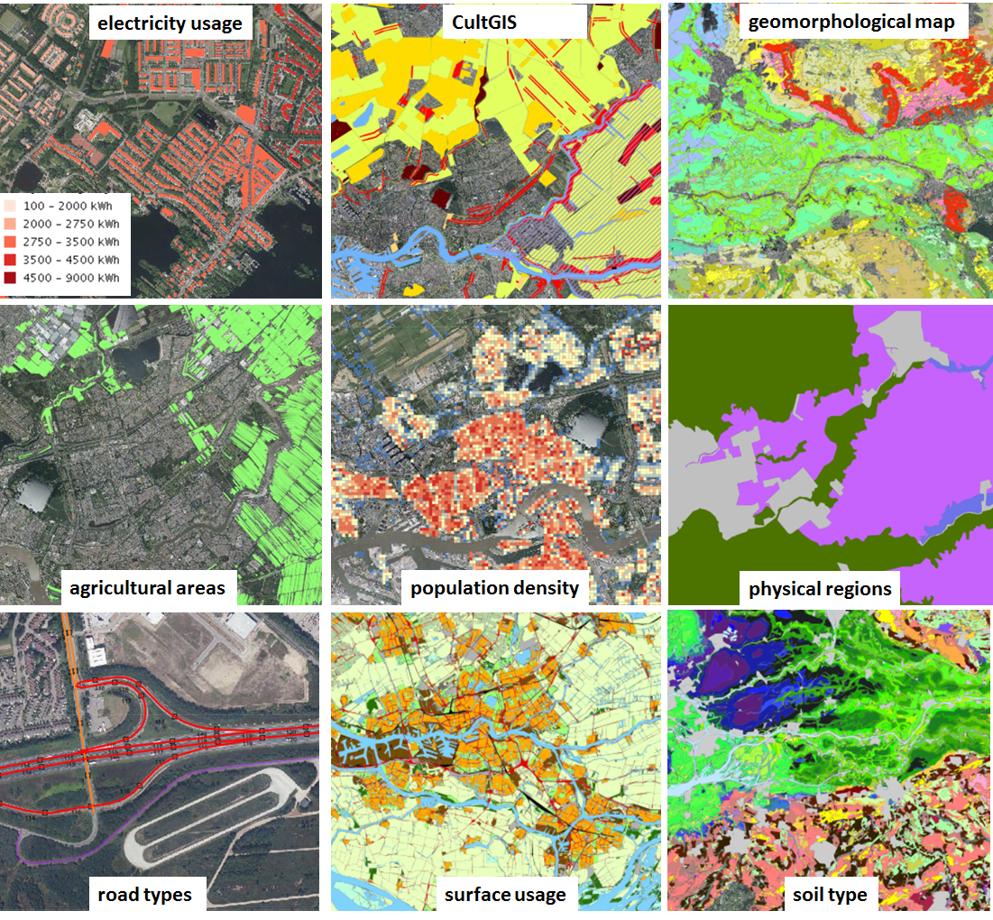 Figure 2: The different types of layers available in PDOK.
So there are many possible datasets you could use as the second layer, and use it to automatically detect these types of features in satellite images.
Another such site containing a lot of maps is the Atlas Natuurlijk Kapitaal.
2.1 Downloading image tiles with owslib
The layer that I am interested in is the layer containing the road-types. The map with the road-types (NWB wegenbestand) can be downloaded from the open data portal of the Dutch government. The aerial images are available as an Web Map Service (WMS) and can be downloaded with the Python package owslib. (The NWB wegenbestand data has been moved from its original location, so I have uploaded it to my dropbox. Same goes for the tiles.)
Below is the code for downloading and saving the image tiles containing aerial photographs with the owslib library.
1
2
3
4
5
6
7
8
9
10
11
12
13
14
15
16
17
18
19
20
21
22
23
24
25
26
27
28
from owslib.wms import WebMapService
URL = "https://geodata.nationaalgeoregister.nl/luchtfoto/rgb/wms?request=GetCapabilities"
wms = WebMapService(URL, version='1.1.1')

OUTPUT_DIRECTORY = './data/image_tiles/'

x_min = 90000
y_min = 427000
dx, dy = 200, 200
no_tiles_x = 100
no_tiles_y = 100
total_no_tiles = no_tiles_x * no_tiles_y

x_max = x_min + no_tiles_x * dx
y_max = y_min + no_tiles_y * dy
BOUNDING_BOX = [x_min, y_min, x_max, y_max]

for ii in range(0,no_tiles_x):
    print(ii)
    for jj in range(0,no_tiles_y):
        ll_x_ = x_min + ii*dx
        ll_y_ = y_min + jj*dy
        bbox = (ll_x_, ll_y_, ll_x_ + dx, ll_y_ + dy)
        img = wms.getmap(layers=['Actueel_ortho25'], srs='EPSG:28992', bbox=bbox, size=(256, 256), format='image/jpeg', transparent=True)
        filename = "{}_{}_{}_{}.jpg".format(bbox[0], bbox[1], bbox[2], bbox[3])
        out = open(OUTPUT_DIRECTORY + filename, 'wb')
        out.write(img.read())
        out.close()
With dx and dy we can adjust the zoom level of the tiles. A values of 200 corresponds roughly with a zoom level of 12, and a value of 100 corresponds roughly with a zoom level of 13. As you can see, the lower-left x and y, and the upper-right x and y coordinates are used in the filename, so we will always know where each tile is located.
This process results in 10.000 tiles within the bounding box ((90000, 427000), (110000, 447000)). These coordinates are given in the rijksdriehoekscoordinaten reference system, and it corresponds with the coordinates ((51.82781, 4.44428), (52.00954, 4.73177)) in the WGS 84 reference system. It covers a few square kilometers in the south of Rotterdam (see Figure 3) and contains both urban as well as non-urban area, i.e. there are enough roads for our convolutional neural network to be trained with.
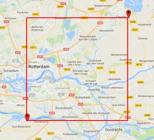 Figure 3: The bounding box of the area we are using to train the ConvNet.
2.2 Reading the shapefile containing the roads of the Netherlands.
Next we will determine the contents of each tile image, using data from the NWB Wegvakken (version September 2017). This is a file containing all of the roads of the Netherlands, which gets updated frequently. It is possible to download it in the form of a shapefile from this location. Shapefiles contain shapes with geospatial data and are normally opened with GIS software like ArcGIS or QGIS. It is also possible to open it within Python, by using the pyshp library.
1
2
3
4
5
6
7
8
9
10
11
12
13
14
15
16
17
18
19
import shapefile
import json

input_filename = './nwb_wegvakken/Wegvakken.shp'
output_filename = './nwb_wegvakken/Wegvakken.json'

reader = shapefile.Reader(shp_filename)
fields = reader.fields[1:]
field_names = [field[0] for field in fields]
buffer = []
for sr in reader.shapeRecords():
    atr = dict(zip(field_names, sr.record))
    geom = sr.shape.__geo_interface__
    buffer.append(dict(type="Feature", geometry=geom, properties=atr))

output_filename = './data/nwb_wegvakken/2017_09_wegvakken.json'
json_file = open(output_filename , "w")
json_file.write(json.dumps({"type": "FeatureCollection", "features": buffer}, indent=2, default=JSONencoder) + "\n")
json_file.close()
In this code, the list ‘buffer’ contains the contents of the shapefile. Since we don’t want to repeat the same shapefile-reading process every time, we will now save it in a json format with json.dumps().
If we try to save the contents of the shapefile as it currently is, it will result in the error '(...) is not JSON Serializable'. This is because the shapefile contains datatypes (bytes and datetime objects) which are not natively supported by JSON. So we need to write an extension to the standard JSON serializer which can take the datatypes not supported by JSON and convert them into datatypes which can be serialized. This is what the method JSONencoder does. (For more on this see here).
1
2
3
4
5
6
7
8
9
10
def JSONencoder(obj):
    """JSON serializer for objects not serializable by default json code"""

    if isinstance(obj, (datetime, date)):
        serial = obj.isoformat()
        return serial
    if isinstance(obj, bytes):
        return {'__class__': 'bytes',
                '__value__': list(obj)}
    raise TypeError ("Type %s not serializable" % type(obj))
If we look at the contents of this shapefile, we will see that it contains a list of objects of the following type:
1
2
3
4
5
6
7
8
9
10
{'properties': {'E_HNR_LNKS': 1, 'WEGBEHSRT': 'G', 'EINDKM': None, 'RIJRICHTNG': '', 'ROUTELTR4': '',
'ROUTENR3': None, 'WEGTYPE': '', 'ROUTENR': None, 'GME_ID': 717, 'ADMRICHTNG': '', 'WPSNAAMNEN': 'DOMBURG', 'DISTRCODE': 0,
'WVK_BEGDAT': '1998-01-21', 'WGTYPE_OMS': '', 'WEGDEELLTR': '#', 'HNRSTRRHTS': '', 'WEGBEHNAAM': 'Veere', 'JTE_ID_BEG': 47197012,
'DIENSTNAAM': '', 'WVK_ID': 47197071, 'HECTO_LTTR': '#', 'RPE_CODE': '#', 'L_HNR_RHTS': None, 'ROUTELTR3': '',
'WEGBEHCODE': '717', 'ROUTELTR': '', 'GME_NAAM': 'Veere', 'L_HNR_LNKS': 11, 'POS_TV_WOL': '', 'BST_CODE': '',
'BEGINKM': None, 'ROUTENR2': None, 'DISTRNAAM': '', 'ROUTELTR2': '', 'WEGNUMMER': '', 'ENDAFSTAND': None, 'E_HNR_RHTS': None,
'ROUTENR4': None, 'BEGAFSTAND': None, 'DIENSTCODE': '', 'STT_NAAM': 'Van Voorthuijsenstraat', 'WEGNR_AW': '',
'HNRSTRLNKS': 'O', 'JTE_ID_END': 47197131}, 'type': 'Feature',
'geometry': {'coordinates': [[23615.0, 398753.0], [23619.0, 398746.0], [23622.0, 398738.0], [23634.0, 398692.0]],
'type': 'LineString'}}
It contains a lot of information (and what each of them means is specified in the manual), but what is of immediate importance to us, are the values of
- ‘WEGBEHSRT’ –> This indicates the road-type
- ‘coordinates’ –> These are the coordinates of this specific object given in the ‘rijkscoordinaten’ system.
The different road-types present in NWB Wegvakken are: 
3. Mapping the two layers of data
Now it is time to determine which tiles contain roads, and which tiles do not. We will do this by mapping the contents of NWB-Wegvakken on top of the downloaded aerial photograph tiles. We can use a Python dictionary to keep track of the mappings. We will also use an dictionary to keep track of the types of road present in each tile.
1
2
3
4
5
6
7
8
9
10
11
12
13
14
15
16
17
18
19
20
21
22
23
24
25
26
27
28
29
30
31
32
33
34
#First we define some variables, and dictionary keys which are going to be used throughout the rest.
dict_roadtype = {
    "G": 'Gemeente',
    "R": 'Rijk',
    "P": 'Provincie',
    "W": 'Waterschap',
    'T': 'Andere wegbeheerder',
    '' : 'leeg'
}

dict_roadtype_to_color = {
    "G": 'red',
    "R": 'blue',
    "P": 'green',
    "W": 'magenta',
    'T': 'yellow',
    '' : 'leeg'
}

FEATURES_KEY = 'features'
PROPERTIES_KEY = 'properties'
GEOMETRY_KEY = 'geometry'
COORDINATES_KEY = 'coordinates'
WEGSOORT_KEY = 'WEGBEHSRT'

MINIMUM_NO_POINTS_PER_TILE = 4
POINTS_PER_METER = 0.1

INPUT_FOLDER_TILES = './data/image_tiles/'

filename_wegvakken = './data/nwb_wegvakken/2017_09_wegvakken.json'
dict_nwb_wegvakken = json.load(open(filename_wegvakken))[FEATURES_KEY]
d_tile_contents = defaultdict(list)
d_roadtype_tiles = defaultdict(set)
In the code above, the contents of NWB wegvakken, which we have previously converted from a Shapefile to a .JSON format are loaded into dict_nwb_wegvakken.
Furthermore, we initialize two defaultdicts. The first one will be filled with the tiles as the keys, and a list of its contents as the values. The second dictionary will be filled with the road-type as the keys, and all tiles containing these road-types as the values. How this is done, is shown below:
1
2
3
4
5
6
7
8
9
10
11
12
13
14
15
16
17
18
19
for elem in dict_nwb_wegvakken:
    coordinates = retrieve_coordinates(elem)
    rtype = retrieve_roadtype(elem)
    coordinates_in_bb = [coord for coord in coordinates if coord_is_in_bb(coord, BOUNDING_BOX)]
    if len(coordinates_in_bb)==1:
        coord = coordinates_in_bb[0]
        add_to_dict(d_tile_contents, d_roadtype_tiles, coord, rtype)
    if len(coordinates_in_bb)>1:
        add_to_dict(d_tile_contents, d_roadtype_tiles, coordinates_in_bb[0], rtype)
        for ii in range(1,len(coordinates_in_bb)):
            previous_coord = coordinates_in_bb[ii-1]
            coord = coordinates_in_bb[ii]
            add_to_dict(d_tile_contents, d_roadtype_tiles, coord, rtype)

            dist = eucledian_distance(previous_coord, coord)
            no_intermediate_points = int(dist/10)
            intermediate_coordinates = calculate_intermediate_points(previous_coord, coord, no_intermediate_points)
            for intermediate_coord in intermediate_coordinates:
                add_to_dict(d_tile_contents, d_roadtype_tiles, intermediate_coord, rtype)
As you can see, we iterate over the contents of dict_nwb_wegvakken, and for each element, we look up the coordinates and the road-types and check which of these coordinates are inside our bounding box. This is done with the following methods:
1
2
3
4
5
6
7
8
9
10
11
12
13
14
15
16
17
18
19
20
21
22
23
24
25
def coord_is_in_bb(coord, bb):
    x_min = bb[0]
    y_min = bb[1]
    x_max = bb[2]
    y_max = bb[3]
    return coord[0] > x_min and coord[0] < x_max and coord[1] > y_min and coord[1] < y_max

def retrieve_roadtype(elem):
    return elem[PROPERTIES_KEY][WEGSOORT_KEY]

def retrieve_coordinates(elem):
    return elem[GEOMETRY_KEY][COORDINATES_KEY]

def add_to_dict(d1, d2, coordinates, rtype):
    coordinate_ll_x = int((coordinates[0] // dx)*dx)
    coordinate_ll_y = int((coordinates[1] // dy)*dy)
    coordinate_ur_x = int((coordinates[0] // dx)*dx + dx)
    coordinate_ur_y = int((coordinates[1] // dy)*dy + dy)
    tile = "{}_{}_{}_{}.jpg".format(coordinate_ll_x, coordinate_ll_y, coordinate_ur_x, coordinate_ur_y)

    rel_coord_x = (coordinates[0] - coordinate_ll_x) / dx
    rel_coord_y = (coordinates[1] - coordinate_ll_y) / dy
    value = (rtype, rel_coord_x, rel_coord_y)
    d1[tile].append(value)
    d2[rtype].add(tile)
As you can see, the add_to_dict method first determines to which tile a coordinate belongs to, by determining the four coordinates (lowerleft x, y and upperright x,y) each tile is named with. We also determine the relative position of each coordinate in its tile. The coordinate (99880, 445120) in tile “99800_445000_100000_445200.jpg” will for example have relative coordinates (0.4, 0.6). This is handy later on when you want to plot the contents of a tile. The road-type, together with the relative coordinate are appended to the list of contents of the tile. At the same time, we add the tilename to the second dictionary which contains a list of tilenames per road-type.
- If there is only one set of coordinates, and these coordinates are inside our bounding box, we immediately add these coordinate to our dictionaries.
- If there are more than one coordinate in an element, we do not only add all coordinates to the dictionaries, but also calculate all intermediate points between two subsequent coordinates and add these intermediate points to the dictionaries. This is necessary because two coordinates could form a shape/line which describes a road which lies inside a tile, but if the coordinates happen to lie outside of the tile, we will think this tile does not contain any road. This is illustrated in Figure 4. On the left we can see two points describing a road, but they happen to lie outside of the tile, and on the right we also calculate every intermediate point (every 1/POINTS_PER_METER meter) between two points and add the intermediate points to the dictionary.
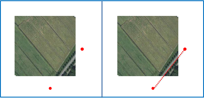 Figure 4: By also using calculated intermediate points we are making sure that we take every part of the road into account.
3.2 Visualizing the Mapping results
It is always good to make visualizations. It gives us an indication if the mapping of points on the tiles went correctly, whether we have missed any roads, and if we have chosen enough intermediate points between two coordinates to fully cover all parts of the roads.
1
2
3
4
5
6
7
8
9
10
11
12
13
14
15
16
17
18
19
20
21
22
23
24
25
26
27
fig, axarr = plt.subplots(nrows=11,ncols=11, figsize=(16,16))

for ii in range(0,11):
    for jj in range(0,11):
        ll_x = x0 + ii*dx
        ll_y = y0 + jj*dy
        ur_x = ll_x + dx
        ur_y = ll_y + dy
        tile = "{}_{}_{}_{}.jpg".format(ll_x, ll_y, ur_x, ur_y)
        filename = INPUT_FOLDER_TILES + tile
        tile_contents = d_tile_contents[tile]

        ax = axarr[10-jj, ii]
        image = ndimage.imread(filename)
        rgb_image = cv2.cvtColor(image, cv2.COLOR_BGR2RGB)
        ax.imshow(rgb_image)
        ax.get_xaxis().set_visible(False)
        ax.get_yaxis().set_visible(False)

        for elem in tile_contents:
            color = dict_roadtype_to_color[elem[0]]
            x = elem[1]*256
            y = (1-elem[2])*256
            ax.scatter(x,y,c=color,s=10)

plt.subplots_adjust(wspace=0, hspace=0)
plt.show()
In Figure 5, we can see two figures, on the left for (x0 = 94400, y0 = 432000) and on the right for (x0 = 93000, y0 = 430000). You can click on them for a larger view.
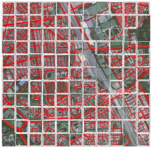
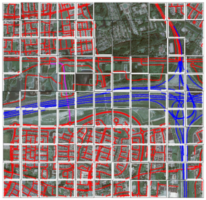 Figure 5: Two figures with the result of the mapping of NWB wegenbestand on top of the tiles.
4. Detecting roads with the convolutional neural network
4.1 Preparing a training, test and validation dataset
Next we will load all of the tiles together with their correct labels (road-presence and/or road-type) into a dataset. The dataset is randomized and then split in a training, test and validation part.
1
2
3
4
5
6
7
8
9
10
11
12
13
14
15
16
17
18
19
20
21
22
23
24
25
26
27
28
image_width = 256
image_height = 256
image_depth = 3
total_no_images = 10000

image_files = os.listdir(INPUT_FOLDER_TILES)

dataset = np.ndarray(shape=(total_no_images, image_width, image_height, image_depth), dtype=np.float32)
labels_roadtype = []
labels_roadpresence = np.ndarray(total_no_images, dtype=np.float32)

for counter, image in enumerate(image_files):
    filename = INPUT_FOLDER_TILES + image
    if image in list(d_tile_contents.keys()):
        tile_contents = d_tile_contents[image]
        roadtypes = sorted(list(set([elem[0] for elem in tile_contents])))
        roadtype = "_".join(roadtypes)
        labels_roadpresence[counter] = 1
    else:
        roadtype = ''
        labels_roadpresence[counter] = 0
    labels_roadtype.append(roadtype)

    image_data = ndimage.imread(filename).astype(np.float32)
    dataset[counter, :, :] = image_data

labels_roadtype_ohe = np.array(list(onehot_encode_labels(labels_roadtype)))
dataset, labels_roadpresence, labels_roadtype_ohe = reformat_data(dataset, labels_roadpresence, labels_roadtype_ohe)
We can use the following functions to one-hot encode the labels, and randomize the dataset:
1
2
3
4
5
6
7
8
9
10
11
12
13
14
15
16
17
18
19
20
21
22
def onehot_encode_labels(labels):
    list_possible_labels = list(np.unique(labels))
    encoded_labels = map(lambda x: list_possible_labels.index(x), labels)
    return encoded_labels

def randomize(dataset, labels1, labels2):
    permutation = np.random.permutation(dataset.shape[0])
    randomized_dataset = dataset[permutation, :, :, :]
    randomized_labels1 = labels1[permutation]
    randomized_labels2 = labels2[permutation]
    return randomized_dataset, randomized_labels1, randomized_labels2

def one_hot_encode(np_array, num_unique_labels):
    return (np.arange(num_unique_labels) == np_array[:,None]).astype(np.float32)

def reformat_data(dataset, labels1, labels2):
    dataset, labels1, labels2 = randomize(dataset, labels1, labels2)
    num_unique_labels1 = len(np.unique(labels1))
    num_unique_labels2 = len(np.unique(labels2))
    labels1 = one_hot_encode(labels1, num_unique_labels1)
    labels2 = one_hot_encode(labels2, num_unique_labels2)
    return dataset, labels1, labels2
4.2 Saving the datasets as a pickle file
This whole process of loading the dataset into memory, and especially randomizing the order of the images usually takes a really long time. So after you have done it once, you want to save the result as a pickle file.
1
2
3
4
5
6
7
8
9
10
11
12
13
14
15
16
17
18
19
20
21
22
23
start_train_dataset = 0
start_valid_dataset = 1200
start_test_dataset = 1600
total_no_images = 2000

output_pickle_file = './data/sattelite_dataset.pickle'

f = open(output_pickle_file, 'wb')
save = {
'train_dataset': dataset[start_train_dataset:start_valid_dataset,:,:,:],
'train_labels_roadtype': labels_roadtype[start_train_dataset:start_valid_dataset],
'train_labels_roadpresence': labels_roadpresence[start_train_dataset:start_valid_dataset],
'valid_dataset': dataset[start_valid_dataset:start_test_dataset,:,:,:],
'valid_labels_roadtype': labels_roadtype[start_valid_dataset:start_test_dataset],
'valid_labels_roadpresence': labels_roadpresence[start_valid_dataset:start_test_dataset],
'test_dataset': dataset[start_test_dataset:total_no_images,:,:,:],
'test_labels_roadtype': labels_roadtype[start_test_dataset:total_no_images],
'test_labels_roadpresence': labels_roadpresence[start_test_dataset:total_no_images],
}
pickle.dump(save, f, pickle.HIGHEST_PROTOCOL)
f.close()

print("\nsaved dataset to {}".format(output_pickle_file))
Now that we have saved the training, validation and test set in a pickle file, we are finished with the preparation part. We can load this pickle file into convolutional neural network and train it to recognize roads.
4.3 Training a convolutional neural network
To train the convolutional neural network to recognize roads, we are going to reuse code from the previous blog post. So if you want to understand how a convolutional neural network actually works, I advise you to take a few minutes and read it.
As you have seen, before we can even start with the CNN, we had to do a lot of work getting and preparing the dataset. This also reflects how data science is in real life; 70 to 80 percent of the time goes into getting, understanding and cleaning data. The actual modelling / training of the data is only a small part of the work.
First we load the dataset from the saved pickle file, import VGGNet from the cnn_models module (see GitHub) and some utility functions (to determine the accuracy) and set the values for the learning rate, batch size, etc.
1
2
3
4
5
6
7
8
9
10
11
12
13
14
15
16
17
18
19
20
21
22
23
24
import pickle
import tensorflow as tf
from cnn_models.vggnet import *
from utils import *

pickle_file = './data/sattelite_dataset.pickle'
f = open(pickle_file, 'rb')
save = pickle.load(f)

train_dataset = save['train_dataset'].astype(dtype = np.float32)
train_labels = save['train_labels_roadpresence'].astype(dtype = np.float32)
test_dataset = save['test_dataset'].astype(dtype = np.float32)
test_labels = save['test_labels_roadpresence'].astype(dtype = np.float32)
valid_dataset = save['valid_dataset'].astype(dtype = np.float32)
valid_labels = save['valid_labels_roadpresence'].astype(dtype = np.float32)

f.close()

num_labels = len(np.unique(train_labels))
num_steps = 501
display_step = 10
batch_size = 16
learning_rate = 0.0001
lambda_loss_amount = 0.0015
After that we can construct the Graph containing all of the computational steps of the Convolutional Neural Network and run it. As you can see, we are using the VGGNet-16 Convolutional Neural Network, l2-regularization to minimize the error, and learning rate of 0.0001. At each step the training accuracy is appended to train_accuracies, and at every 10th step the test and validation accuracies are appended to similar lists. We will use these later to visualize our accuracies.
1
2
3
4
5
6
7
8
9
10
11
12
13
14
15
16
17
18
19
20
21
22
23
24
25
26
27
28
29
30
31
32
33
34
35
36
37
38
39
40
41
42
43
44
45
46
47
48
49
50
51
52
53
54
55
56
57
58
59
60
61
62
63
64
65
66
67
68
69
70
train_accuracies, test_accuracies, valid_accuracies = [], [], []

print("STARTING WITH SATTELITE")
graph = tf.Graph()
with graph.as_default():
    #1) First we put the input data in a tensorflow friendly form.
    tf_train_dataset = tf.placeholder(tf.float32, shape=(batch_size, image_width, image_height, image_depth))
    tf_train_labels = tf.placeholder(tf.float32, shape = (batch_size, num_labels))
    tf_test_dataset = tf.placeholder(tf.float32, shape=(batch_size, image_width, image_height, image_depth))
    tf_test_labels = tf.placeholder(tf.float32, shape = (batch_size, num_labels))
    tf_valid_dataset = tf.placeholder(tf.float32, shape=(batch_size, image_width, image_height, image_depth))
    tf_valid_labels = tf.placeholder(tf.float32, shape = (batch_size, num_labels))

    #2) Then, the weight matrices and bias vectors are initialized
    variables = variables_vggnet16()

    #3. The model used to calculate the logits (predicted labels)
    model = model_vggnet16

    logits = model(tf_train_dataset, variables)

    #4. then we compute the softmax cross entropy between the logits and the (actual) labels
    l2 = lambda_loss_amount * sum(tf.nn.l2_loss(tf_var) for tf_var in tf.trainable_variables())
    loss = tf.reduce_mean(tf.nn.softmax_cross_entropy_with_logits(logits=logits, labels=tf_train_labels)) + l2

    #learning_rate = tf.train.exponential_decay(0.05, global_step, 1000, 0.85, staircase=True)
    #5. The optimizer is used to calculate the gradients of the loss function
    optimizer = tf.train.AdamOptimizer(learning_rate=learning_rate).minimize(loss)

    # Predictions for the training, validation, and test data.
    train_prediction = tf.nn.softmax(logits)
    test_prediction = tf.nn.softmax(model(tf_test_dataset, variables))
    valid_prediction = tf.nn.softmax(model(tf_valid_dataset, variables))

with tf.Session(graph=graph) as session:
    test_counter = 0
    tf.global_variables_initializer().run()
    print('Initialized with learning_rate', learning_rate, " model ", ii)
    for step in range(num_steps):
        #Since we are using stochastic gradient descent, we are selecting  small batches from the training dataset,
        #and training the convolutional neural network each time with a batch.
        offset = (step * batch_size) % (train_labels.shape[0] - batch_size)
        batch_data = train_dataset[offset:(offset + batch_size), :,  :]
        batch_labels = train_labels[offset:(offset + batch_size), :]
        feed_dict = {tf_train_dataset : batch_data, tf_train_labels : batch_labels}

        _, l, predictions = session.run([optimizer, loss, train_prediction], feed_dict=feed_dict)
        train_accuracy = accuracy(predictions, batch_labels)
        train_accuracies.append(train_accuracy)

        if step % display_step == 0:
            offset2 = (test_counter * batch_size) % (test_labels.shape[0] - batch_size)
            test_dataset_batch = test_dataset[offset2:(offset2 + batch_size), :, :]
            test_labels_batch = test_labels[offset2:(offset2 + batch_size), :]
            feed_dict2 = {tf_test_dataset : test_dataset_batch, tf_test_labels : test_labels_batch}

            test_prediction_ = session.run(test_prediction, feed_dict=feed_dict2)
            test_accuracy = accuracy(test_prediction_, test_labels_batch)
            test_accuracies.append(test_accuracy)

            valid_dataset_batch = valid_dataset[offset2:(offset2 + batch_size), :, :]
            valid_labels_batch = valid_labels[offset2:(offset2 + batch_size), :]
            feed_dict3 = {tf_valid_dataset : valid_dataset_batch, tf_valid_labels : valid_labels_batch}

            valid_prediction_ = session.run(valid_prediction, feed_dict=feed_dict3)
            valid_accuracy = accuracy(valid_prediction_, valid_labels_batch)
            valid_accuracies.append(valid_accuracy)

            message = "step {:04d} : loss is {:06.2f}, accuracy on training set {:02.2f} %, accuracy on test set {:02.2f} accuracy on valid set {:02.2f} %".format(step, l, train_accuracy, test_accuracy, valid_accuracy)
            print(message)
Again, if you do not fully understand what is happening here, you can have a look at the previous blog post in which we looked at building Convolutional Neural Networks in Tensorflow in more detail.
4.5 Resulting Accuracy
Below we can see the accuracy results of the convolutional neural network. As you can see, the accuracy for the test as well as the validation set lies around 80 %.
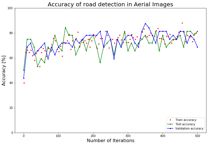 Figure 6: Accuracy on the training, test and validation set.
If we look at the tiles which have been classified inaccurately, we can see that most of these tiles are classified wrongly because it really is difficult to detect the roads on these images.
 Figure 7: Some of the tiles which were wrongly classified.
5. Final Words
We have seen how we can detect roads in satellite or aerial images using CNNs. Although it is quite amazing what you can do with Convolutional Neural Networks, the technical development in A.I. and Deep Learning world is so fast that using ‘only a CNN’ is already outdated.
- Since a few years there are also Neural Networks called R-CNN, Fast R-CNN and Faster R-CNN (like SSD, YOLO and YOLO9000). These Neural Networks can not only detect the presence of objects in images, but also return the bounding boxes of the object.
- Nowadays there are also Neural Networks which can perform segmentation tasks (like DeepMask, SharpMask, MultiPath), i.e. they can determine to which object each pixel in the image belongs.
I think these Neural Networks which can perform image segmentation would be ideal to determine the location of roads and other objects inside satellite images. In future blogs, I want to have a look at how we can detect roads (or other features) in satellite and aerial images using these types of Neural Networks.
If you are interested in the latest developments in Computer Vision, I can recommend you to read a year in computer vision.