update: The code presented in this blog-post is also available in my GitHub repository.
update2: I have added sections 2.4 , 3.2 , 3.3.2 and 4 to this blog post, updated the code on GitHub and improved upon some methods.
1. Introduction
For python programmers, scikit-learn is one of the best libraries to build Machine Learning applications with. It is ideal for beginners because it has a really simple interface, it is well documented with many examples and tutorials.
Besides supervised machine learning (classification and regression), it can also be used for clustering, dimensionality reduction, feature extraction and engineering, and pre-processing the data. The interface is consistent over all of these methods, so it is not only easy to use, but it is also easy to construct a large ensemble of classifiers/regression models and train them with the same commands.
In this blog lets have a look at how to build, train, evaluate and validate a classifier with scikit-learn, improve upon the initial classifier with hyper-parameter optimization and look at ways in which we can have a better understanding of complex datasets.
We will do this by going through the of classification of two example datasets. The glass dataset, and the Mushroom dataset.
The glass dataset contains data on six types of glass (from building windows, containers, tableware, headlamps, etc) and each type of glass can be identified by the content of several minerals (for example Na, Fe, K, etc). This dataset only contains numerical data and therefore is a good dataset to get started with.
The second dataset contains non-numerical data and we will need an additional step where we encode the categorical data to numerical data.
2. Classification of the glass dataset:
Lets start with classifying the classes of glass!
First we need to import the necessary modules and libraries which we will use.
|
1 2 3 4 5 6 7 8 9 10 11 12 13 14 15 16 17 18 19 |
import pandas as pd import numpy as np import seaborn as sns import matplotlib.pyplot as plt import time from sklearn.decomposition import PCA from sklearn.preprocessing import StandardScaler, LabelEncoder from sklearn.linear_model import LogisticRegression from sklearn.svm import SVC from sklearn.neighbors import KNeighborsClassifier from sklearn import tree from sklearn.neural_network import MLPClassifier from sklearn.neighbors import KNeighborsClassifier from sklearn.ensemble import GradientBoostingClassifier from sklearn.gaussian_process.kernels import RBF from sklearn.ensemble import RandomForestClassifier from sklearn.naive_bayes import GaussianNB |
- The pandas module is used to load, inspect, process the data and get in the shape necessary for classification.
- Seaborn is a library based on matplotlib and has nice functionalities for drawing graphs.
- StandardScaler is a library for standardizing and normalizing dataset and
- the LaberEncoder library can be used to One Hot Encode the categorical features (in the mushroom dataset).
- All of the other modules are classifiers which are used for classification of the dataset.
2.1 Loading, analyzing and processing the dataset:
When loading a dataset for the first time, there are several questions we need to ask ourself:
- What kind of data does the dataset contain? Numerical data, categorical data, geographic information, etc…
- Does the dataset contain any missing data?
- Does the dataset contain any redundant data (noise)?
- Do the values of the features differ over many orders of magnitude? Do we need to standardize or normalize the dataset?
|
1 2 3 4 5 6 |
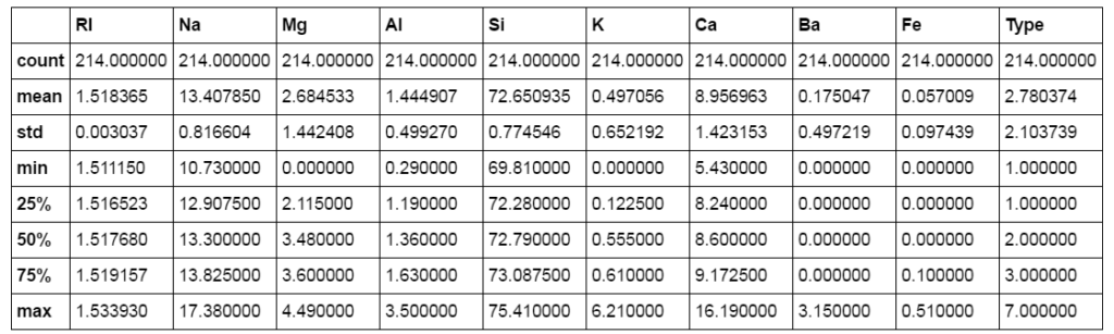
filename_glass = './data/glass.csv' df_glass = pd.read_csv(filename_glass) print(df_glass.shape) display(df_glass.head()) display(df_glass.describe()) |
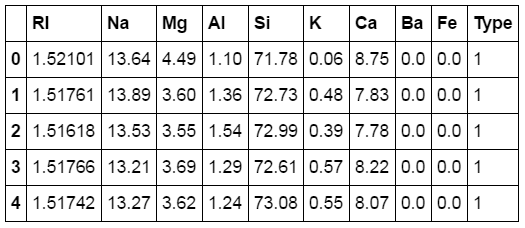
We can see that the dataset consists of 214 rows and 10 columns. All of the columns contain numerical data, and there are no rows with missing information. Also most of the features have values in the same order of magnitude.
So for this dataset we do not need to remove any rows, impute missing values or transform categorical data into numerical.
The .describe() method we used above is useful for giving a quick overview of the dataset;
- How many rows of data are there?
- What are some characteristic values like the mean, standard deviation, minimum and maximum value, the 25th percentile etc.
2.3 Classification and validation
The next step is building and training the actual classifier, which hopefully can accurately classify the data. With this we will be able to tell which type of glass an entry in the dataset belongs to, based on the features.
For this we need to split the dataset into a training set and a test set. With the training set we will train the classifier, and with the test set we will validate the accuracy of the classifier. Usually a 70 % / 30 % ratio is used when splitting into a training and test set, but this ratio should be chosen based on the size of the dataset. For example, if the dataset does not have enough entries, 30% of it might not contain all of the classes or enough information to properly function as a validation set.
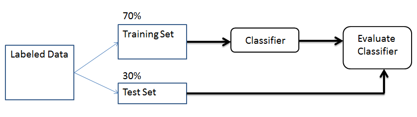
Another important note is that the distribution of the different classes in both the training and the test set should be equal to the distribution in the actual dataset. For example, if you have a dataset with review-texts which contains 20% negative and 80% positive reviews, both the training and the test set should have this 20% / 80% ratio. The best way to do this, is to split the dataset into a training and test set randomly.
|
1 2 3 4 5 6 7 8 9 10 11 12 13 14 15 16 17 18 19 20 21 22 |
def get_train_test(df, y_col, x_cols, ratio): """ This method transforms a dataframe into a train and test set, for this you need to specify: 1. the ratio train : test (usually 0.7) 2. the column with the Y_values """ mask = np.random.rand(len(df)) < ratio df_train = df[mask] df_test = df[~mask] Y_train = df_train[y_col].values Y_test = df_test[y_col].values X_train = df_train[x_cols].values X_test = df_test[x_cols].values return df_train, df_test, X_train, Y_train, X_test, Y_test y_col_glass = 'Type' x_cols_glass = list(df_glass.columns.values) x_cols_glass.remove(y_col_glass) train_test_ratio = 0.7 df_train, df_test, X_train, Y_train, X_test, Y_test = get_train_test(df_glass, y_col_glass, x_cols_glass, train_test_ratio) |
With the dataset splitted into a training and test set, we can start building a classification model. We will do this in a slightly different way as usual. The idea behind this is that, when we start with a new dataset, we don’t know which (type of) classifier will perform best on this dataset. Will it be a ensemble classifier like Gradient Boosting or Random Forest, or a classifier which uses a functional approach like Logistic Regression, a classifier which uses a statistical approach like Naive Bayes etc.?
Because we dont know this, and nowadays computational power is cheap to get, we will try out all types of classifiers first and later we can continue to optimize the best performing classifier of this inital batch of classifiers. For this we have to make an dictionary, which contains as keys the name of the classifiers and as values an instance of the classifiers.
|
1 2 3 4 5 6 7 8 9 10 11 12 13 |
dict_classifiers = { "Logistic Regression": LogisticRegression(), "Nearest Neighbors": KNeighborsClassifier(), "Linear SVM": SVC(), "Gradient Boosting Classifier": GradientBoostingClassifier(n_estimators=1000), "Decision Tree": tree.DecisionTreeClassifier(), "Random Forest": RandomForestClassifier(n_estimators=1000), "Neural Net": MLPClassifier(alpha = 1), "Naive Bayes": GaussianNB(), #"AdaBoost": AdaBoostClassifier(), #"QDA": QuadraticDiscriminantAnalysis(), #"Gaussian Process": GaussianProcessClassifier() } |
Then we can iterate over this dictionary, and for each classifier:
- train the classifier with
.fit(X_train, Y_train) - evaluate how the classifier performs on the training set with
.score(X_train, Y_train) - evaluate how the classifier perform on the test set with
.score(X_test, Y_test). - keep track of how much time it takes to train the classifier with the time module.
- save the trained model, the training score, the test score, and the training time into a dictionary. If necessary this dictionary can be saved with Python’s pickle module.
|
1 2 3 4 5 6 7 8 9 10 11 12 13 14 15 16 17 18 19 20 21 22 23 24 25 26 27 28 29 30 31 32 33 34 35 36 37 38 39 40 41 42 43 |
def batch_classify(X_train, Y_train, X_test, Y_test, no_classifiers = 5, verbose = True): """ This method, takes as input the X, Y matrices of the Train and Test set. And fits them on all of the Classifiers specified in the dict_classifier. The trained models, and accuracies are saved in a dictionary. The reason to use a dictionary is because it is very easy to save the whole dictionary with the pickle module. Usually, the SVM, Random Forest and Gradient Boosting Classifier take quiet some time to train. So it is best to train them on a smaller dataset first and decide whether you want to comment them out or not based on the test accuracy score. """ dict_models = {} for classifier_name, classifier in list(dict_classifiers.items())[:no_classifiers]: t_start = time.clock() classifier.fit(X_train, Y_train) t_end = time.clock() t_diff = t_end - t_start train_score = classifier.score(X_train, Y_train) test_score = classifier.score(X_test, Y_test) dict_models[classifier_name] = {'model': classifier, 'train_score': train_score, 'test_score': test_score, 'train_time': t_diff} if verbose: print("trained {c} in {f:.2f} s".format(c=classifier_name, f=t_diff)) return dict_models def display_dict_models(dict_models, sort_by='test_score'): cls = [key for key in dict_models.keys()] test_s = [dict_models[key]['test_score'] for key in cls] training_s = [dict_models[key]['train_score'] for key in cls] training_t = [dict_models[key]['train_time'] for key in cls] df_ = pd.DataFrame(data=np.zeros(shape=(len(cls),4)), columns = ['classifier', 'train_score', 'test_score', 'train_time']) for ii in range(0,len(cls)): df_.loc[ii, 'classifier'] = cls[ii] df_.loc[ii, 'train_score'] = training_s[ii] df_.loc[ii, 'test_score'] = test_s[ii] df_.loc[ii, 'train_time'] = training_t[ii] display(df_.sort_values(by=sort_by, ascending=False)) |
The reason why we keep track of the time it takes to train a classifier, is because in practice this is also an important indicator of whether or not you would like to use a specific classifier. If there are two classifiers with similar results, but one of them takes much less time to train you probably want to use that one.
The score() method simply return the result of the accuracy_score() method in the metrics module. This module, contains many methods for evualating classification or regression models and I can recommend you to spent some time to learn which metrics you can use to evaluate your model.
The classification_report method for example, calculates the precision, recall and f1-score for all of the classes in your dataset. If you are looking for ways to improve the accuracy of your classifier, or if you want to know why the accuracy is lower than expected, such detailed information about the performance of the classifier on the dataset can point you in the right direction.
The accuracy on the training set, accuracy on the test set, and the duration of the training was saved into a dictionary, and we can use the display_dict_models() method to visualize the results ordered by the test score.
|
1 2 |
dict_models = batch_classify(X_train, Y_train, X_test, Y_test, no_classifiers = 8) display_dict_models(dict_models) |
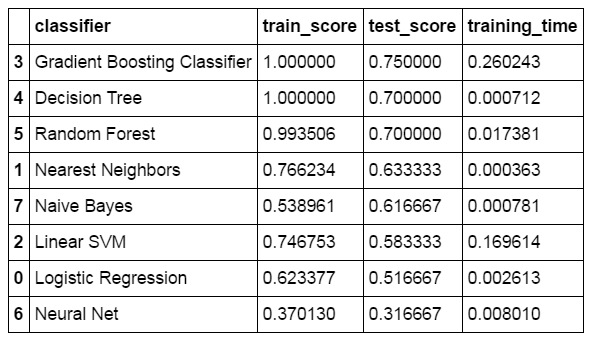
What we are doing feels like a brute force approach, where a large number of classifiers are build to see which one performs best. It gives us an idea which classifier will perform better for a particular dataset and which one will not. After that you can continue with the best (or top 3) classifier, and try to improve the results by tweaking the parameters of the classifier, or by adding more features to the dataset.
As we can see, the Gradient Boosting classifier performs the best for this dataset. Actually, classifiers like Random Forest and Gradient Boosting classification performs best for most datasets and challenges on Kaggle (That does not mean you should rule out all other classifiers).
For the ones who are interested in the theory behind these classifiers, scikit-learn has a pretty well written user guide. Some of these classifiers were also explained in previous posts, like the naive bayes classifier, logistic regression and support vector machines was partially explained in the perceptron blog.
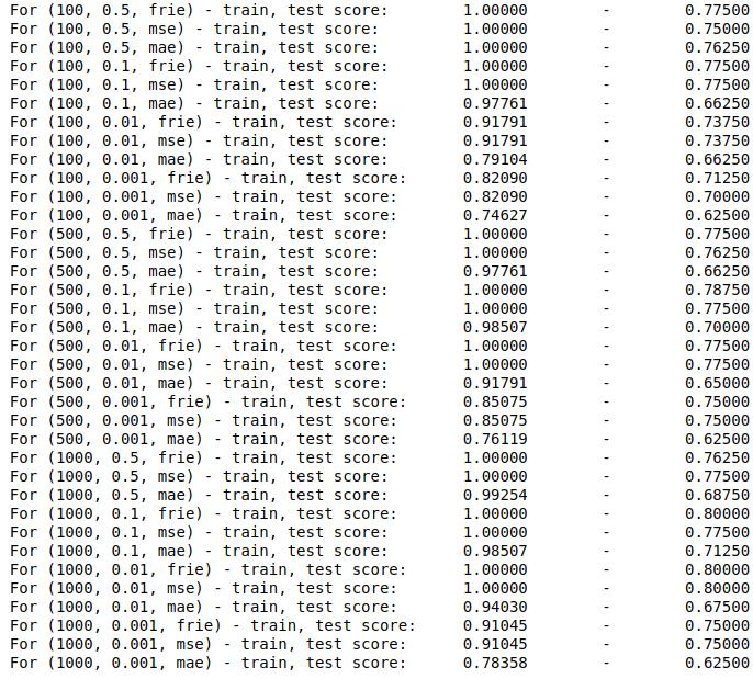
2.4 Improving upon the Classifier: hyperparameter optimization
After we have determined with a quick and dirty method which classifier performs best for the dataset, we can improve upon the Classifier by optimizing its hyper-parameters.
|
1 2 3 4 5 6 7 8 9 10 11 12 13 14 15 16 17 18 |
GDB_params = { 'n_estimators': [100, 500, 1000], 'learning_rate': [0.5, 0.1, 0.01, 0.001], 'criterion': ['friedman_mse', 'mse', 'mae'] } df_train, df_test, X_train, Y_train, X_test, Y_test = get_train_test(df_glass, y_col_glass, x_cols_glass, 0.6) for n_est in GDB_params['n_estimators']: for lr in GDB_params['learning_rate']: for crit in GDB_params['criterion']: clf = GradientBoostingClassifier(n_estimators=n_est, learning_rate = lr, criterion = crit) clf.fit(X_train, Y_train) train_score = clf.score(X_train, Y_train) test_score = clf.score(X_test, Y_test) print("For ({}, {}, {}) - train, test score: \t {:.5f} \t-\t {:.5f}".format(n_est, lr, crit[:4], train_score, test_score)) |
3. Classification of the mushroom dataset:
The second dataset we will have a look at is the mushroom dataset, which contains data on edible vs poisonous mushrooms. In the dataset there are 8124 mushrooms in total (4208 edible and 3916 poisonous) described by 22 features each.
The big difference with the glass dataset is that these features don’t have a numerical, but a categorical value. Because this dataset contains categorical values, we need one extra step in the classification process, which is the encoding of these values (see section 3.3).
3.1 Loading, analyzing and pre-processing the data.
|
1 2 3 |
filename_mushrooms = './data/mushrooms.csv' df_mushrooms = pd.read_csv(filename_mushrooms) display(df_mushrooms.head()) |
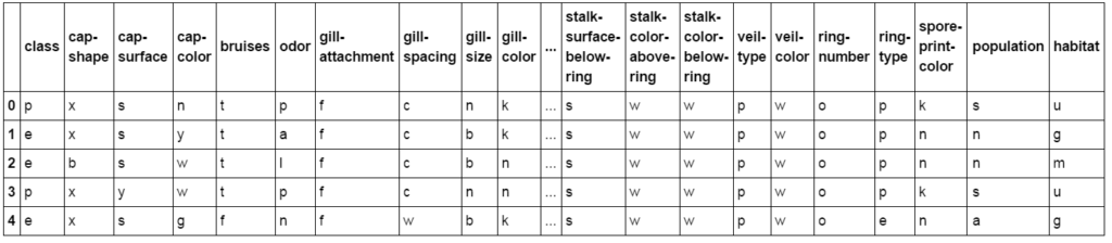
A fast way to find out what type of categorical data a dataset contains, is to print out the unique values of each column in this dataframe. In this way we can also see whether the dataset contains any missing values or redundant columns.
|
1 2 |
for col in df_mushrooms.columns.values: print(col, df_mushrooms[col].unique()) |
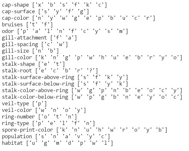
As we can see, there are 22 categorical features. Of these, the feature ‘veil-type’ only contains one value ‘p’ and therefore does not provide any added value for any classifier. The best thing to do is to remove columns like this which only contain one value.
|
1 2 3 |
for col in df_mushrooms.columns.values: if len(df_mushrooms[col].unique()) <= 1: print("Removing column {}, which only contains the value: {}".format(col, df_mushrooms[col].unique()[0])) |
3.2 Imputing Missing values
Some datasets contain missing values in the form of NaN, null, NULL, ‘?’, ‘??’ etc
It could be that all missing values are of type NaN, or that some columns contain NaN and other columns contain missing data in the form of ‘??’.
It is up to your best judgement to decide what to do with these missing values. What is most effective, really depends on the type of data, the type of missing data and the ratio between missing data and non-missing data.
- If the number of rows containing missing data is only a few percent of the total dataset, the best option could be to drop those rows. If half of the rows contain missing values, we could lose valuable information by dropping all of them.
- If there is a row or column which contains almost only missing data, it will not have much added value and it might be best to drop that column.
- It could be that a value not being filled in also is information which helps with the classification and it is best to leave it like it is.
- Maybe we really need to improve the accuracy and the only way to do this is by Imputing the missing values.
- etc, etc
Below we will look at a few ways in which you can either remove the missing values, or impute them.
3.2.1 Drop rows with missing values
|
1 2 3 |
print("Number of rows in total: {}".format(df_mushrooms.shape[0])) print("Number of rows with missing values in column 'stalk-root': {}".format(df_mushrooms[df_mushrooms['stalk-root'] == '?'].shape[0])) df_mushrooms_dropped_rows = df_mushrooms[df_mushrooms['stalk-root'] != '?'] |
3.2.2 Drop column with more than X percent missing values
|
1 2 3 4 5 6 7 8 9 10 11 |
drop_percentage = 0.8 df_mushrooms_dropped_cols = df_mushrooms.copy(deep=True) df_mushrooms_dropped_cols.loc[df_mushrooms_dropped_cols['stalk-root'] == '?', 'stalk-root'] = np.nan for col in df_mushrooms_dropped_cols.columns.values: no_rows = df_mushrooms_dropped_cols[col].isnull().sum() percentage = no_rows / df_mushrooms_dropped_cols.shape[0] if percentage > drop_percentage: del df_mushrooms_dropped_cols[col] print("Column {} contains {} missing values. This is {} percent. Dropping this column.".format(col, no_rows, percentage)) |
3.2.3 Fill missing values with zeros
|
1 2 3 |
df_mushrooms_zerofill = df_mushrooms.copy(deep = True) df_mushrooms_zerofill.loc[df_mushrooms_zerofill['stalk-root'] == '?', 'stalk-root'] = np.nan df_mushrooms_zerofill.fillna(0, inplace=True) |
3.2.4 Fill missing values with backward fill
|
1 2 3 |
df_mushrooms_bfill = df_mushrooms.copy(deep = True) df_mushrooms_bfill.loc[df_mushrooms_bfill['stalk-root'] == '?', 'stalk-root'] = np.nan df_mushrooms_bfill.fillna(method='bfill', inplace=True) |
3.2.5 Fill missing values with forward fill
|
1 2 3 |
df_mushrooms_ffill = df_mushrooms.copy(deep = True) df_mushrooms_ffill.loc[df_mushrooms_ffill['stalk-root'] == '?', 'stalk-root'] = np.nan df_mushrooms_ffill.fillna(method='ffill', inplace=True) |
3.3 Encoding categorical data
Most classifier can only work with numerical data, and will raise an error when categorical values in the form of strings is used as input. When it comes to columns with categorical data, you can do two things.
- 1) One-hot encode the column such that its categorical values are converted to numerical values.
- 2) Expand the column into N different columns containing binary values.
Example: Let assume that we have a column called ‘FRUIT’ which contains the unique values [‘ORANGE’, ‘APPLE’, PEAR’].
- In the first case it would be converted to the unique values [0, 1, 2]
- In the second case it would be converted into three different columns called [‘FRUIT_IS_ORANGE’, ‘FRUIT_IS_APPLE’, ‘FRUIT_IS_PEAR’] and after this the original column ‘FRUIT’ would be deleted. The three new columns would contain the values 1 or 0 depending on the value of the original column.
When using the first method, you should pay attention to the fact that some classifiers will try to make sense of the numerical value of the one-hot encoded column. For example the Nearest Neighbour algorithm assumes that the value 1 is closer to 0 than the value 2. But the numerical values have no meaning in the case of one-hot encoded columns (an APPLE is not closer to an ORANGE than a PEAR is.) and the results therefore can be misleading.
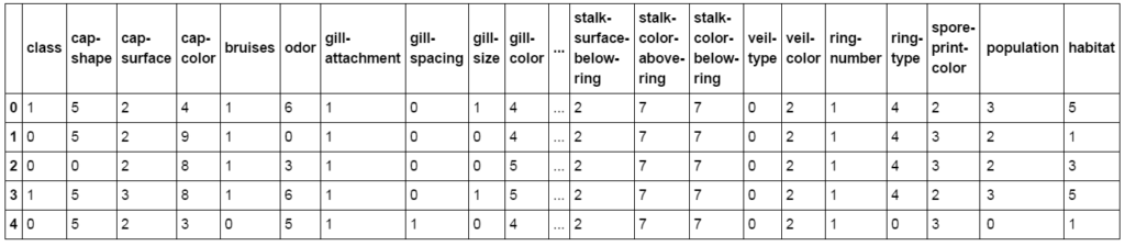
3.3.1 One-Hot encoding the columns with categorical data
|
1 2 3 4 5 6 7 8 9 10 11 12 13 14 15 16 17 18 19 20 21 22 23 24 25 26 27 |
def label_encode(df, columns): for col in columns: le = LabelEncoder() col_values_unique = list(df[col].unique()) le_fitted = le.fit(col_values_unique) col_values = list(df[col].values) le.classes_ col_values_transformed = le.transform(col_values) df[col] = col_values_transformed df_mushrooms_ohe = df_mushrooms.copy(deep=True) to_be_encoded_cols = df_mushrooms_ohe.columns.values label_encode(df_mushrooms_ohe, to_be_encoded_cols) display(df_mushrooms_ohe.head()) ## Now lets do the same thing for the other dataframes df_mushrooms_dropped_rows_ohe = df_mushrooms_dropped_rows.copy(deep = True) df_mushrooms_zerofill_ohe = df_mushrooms_zerofill.copy(deep = True) df_mushrooms_bfill_ohe = df_mushrooms_bfill.copy(deep = True) df_mushrooms_ffill_ohe = df_mushrooms_ffill.copy(deep = True) label_encode(df_mushrooms_dropped_rows_ohe, to_be_encoded_cols) label_encode(df_mushrooms_zerofill_ohe, to_be_encoded_cols) label_encode(df_mushrooms_bfill_ohe, to_be_encoded_cols) label_encode(df_mushrooms_ffill_ohe, to_be_encoded_cols) |
3.3.2 Expanding the columns with categorical data
|
1 2 3 4 5 6 7 8 9 10 11 12 13 14 15 16 17 18 19 20 21 22 23 24 25 26 27 28 29 30 31 32 33 34 |
def expand_columns(df, list_columns): for col in list_columns: colvalues = df[col].unique() for colvalue in colvalues: newcol_name = "{}_is_{}".format(col, colvalue) df.loc[df[col] == colvalue, newcol_name] = 1 df.loc[df[col] != colvalue, newcol_name] = 0 df.drop(list_columns, inplace=True, axis=1) y_col = 'class' to_be_expanded_cols = list(df_mushrooms.columns.values) to_be_expanded_cols.remove(y_col) df_mushrooms_expanded = df_mushrooms.copy(deep=True) label_encode(df_mushrooms_expanded, [y_col]) expand_columns(df_mushrooms_expanded, to_be_expanded_cols) ## Now lets do the same thing for all other dataframes df_mushrooms_dropped_rows_expanded = df_mushrooms_dropped_rows.copy(deep = True) df_mushrooms_zerofill_expanded = df_mushrooms_zerofill.copy(deep = True) df_mushrooms_bfill_expanded = df_mushrooms_bfill.copy(deep = True) df_mushrooms_ffill_expanded = df_mushrooms_ffill.copy(deep = True) label_encode(df_mushrooms_dropped_rows_expanded, [y_col]) label_encode(df_mushrooms_zerofill_expanded, [y_col]) label_encode(df_mushrooms_bfill_expanded, [y_col]) label_encode(df_mushrooms_ffill_expanded, [y_col]) expand_columns(df_mushrooms_dropped_rows_expanded, to_be_expanded_cols) expand_columns(df_mushrooms_zerofill_expanded, to_be_expanded_cols) expand_columns(df_mushrooms_bfill_expanded, to_be_expanded_cols) expand_columns(df_mushrooms_ffill_expanded, to_be_expanded_cols) |
3.4 Classification and Validation
We have seen that there are two different ways to handle columns with categorical data, and many different ways to handle missing values.
Since computation power is cheap, it is easy to try out all of classifiers present on all of the different ways we have imputed missing values.
After we have seen which method and which classifier has the highest accuracy initially we can continue in that direction.
Again, we will split the dataset into a 70% training set and a 30% test set and start training and validating a batch of the eight most used classifiers.
|
1 2 3 4 5 6 7 8 9 10 11 12 13 14 15 16 17 18 19 20 21 22 23 24 25 26 |
dict_dataframes = { "df_mushrooms_ohe": df_mushrooms_ohe, "df_mushrooms_dropped_rows_ohe": df_mushrooms_dropped_rows_ohe, "df_mushrooms_zerofill_ohe": df_mushrooms_zerofill_ohe, "df_mushrooms_bfill_ohe": df_mushrooms_bfill_ohe, "df_mushrooms_ffill_ohe": df_mushrooms_ffill_ohe, "df_mushrooms_expanded": df_mushrooms_expanded, "df_mushrooms_dropped_rows_expanded": df_mushrooms_dropped_rows_expanded, "df_mushrooms_zerofill_expanded": df_mushrooms_zerofill_expanded, "df_mushrooms_bfill_expanded": df_mushrooms_bfill_expanded, "df_mushrooms_ffill_expanded": df_mushrooms_ffill_expanded } y_col = 'class' train_test_ratio = 0.7 for df_key, df in dict_dataframes.items(): x_cols = list(df.columns.values) x_cols.remove(y_col) df_train, df_test, X_train, Y_train, X_test, Y_test = get_train_test(df, y_col, x_cols, train_test_ratio) dict_models = batch_classify(X_train, Y_train, X_test, Y_test, no_classifiers = 8, verbose=False) print() print(df_key) display_dict_models(dict_models) print("-------------------------------------------------------") |
As we can see here, the accuracy of the classifiers for this dataset is actually quiet high.
4. Understanding complex datasets
Some datasets contain a lot of features and it is not immediatly clear which of these features are helping with the Classification / Regression, and which of these features are only adding more noise.
To have a better understanding of how the dataset is made up of its features, we will discuss a few methods which can give more insight in the next few sections.
4.1 The correlation matrix
To get more insight in how (strongly) each feature is correlated with the Type of glass, we can calculate and plot the correlation matrix for this dataset.
|
1 2 3 4 5 |
correlation_matrix = df_glass.corr() plt.figure(figsize=(10,8)) ax = sns.heatmap(correlation_matrix, vmax=1, square=True, annot=True,fmt='.2f', cmap ='GnBu', cbar_kws={"shrink": .5}, robust=True) plt.title('Correlation matrix between the features', fontsize=20) plt.show() |
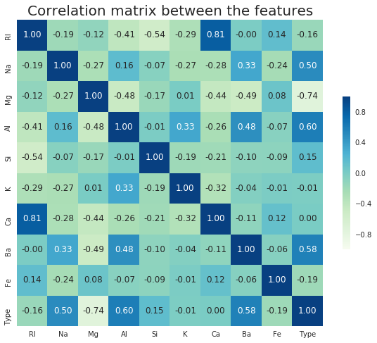
The correlation matrix shows us for example that the oxides ‘Mg’ and ‘Al’ are most strongly correlated with the Type of glass. The content of ‘Ca’ is least strongly correlated with the type of glass. For some dataset there could be features with no correlation at all; then it might be a good idea to remove these since they will only function as noise.
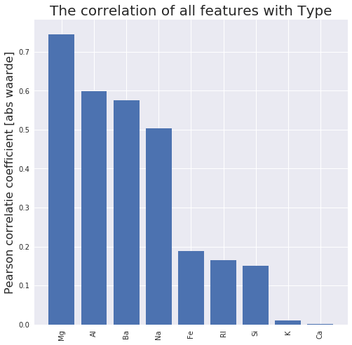
4.2 Correlation of a single feature with other features
A correlation matrix is a good way to get a general picture of how all of features in the dataset are correlated with each other. For a dataset with a lot of features it might become very large and the correlation of a single feature with the other features becomes difficult to discern.
If you want to look at the correlations of a single feature, it usually is a better idea to visualize it in the form of a bar-graph:
|
1 2 3 4 5 6 7 8 9 10 11 12 13 14 15 16 |
def display_corr_with_col(df, col): correlation_matrix = df.corr() correlation_type = correlation_matrix[col].copy() abs_correlation_type = correlation_type.apply(lambda x: abs(x)) desc_corr_values = abs_correlation_type.sort_values(ascending=False) y_values = list(desc_corr_values.values)[1:] x_values = range(0,len(y_values)) xlabels = list(desc_corr_values.keys())[1:] fig, ax = plt.subplots(figsize=(8,8)) ax.bar(x_values, y_values) ax.set_title('The correlation of all features with {}'.format(col), fontsize=20) ax.set_ylabel('Pearson correlatie coefficient [abs waarde]', fontsize=16) plt.xticks(x_values, xlabels, rotation='vertical') plt.show() display_corr_with_col(df_glass, 'Type') |
4.3 Cumulative Explained Variance
The Cumulative explained variance shows how much of the variance is captures by the first x features.
Below we can see that the first 4 features (i.e. the four features with the largest correlation) already capture 90% of the variance.
|
1 2 3 4 5 6 7 8 9 10 11 12 |
X = df_glass[x_cols_glass].values X_std = StandardScaler().fit_transform(X) pca = PCA().fit(X_std) var_ratio = pca.explained_variance_ratio_ components = pca.components_ #print(pca.explained_variance_) plt.plot(np.cumsum(var_ratio)) plt.xlim(0,9,1) plt.xlabel('Number of Features', fontsize=16) plt.ylabel('Cumulative explained variance', fontsize=16) plt.show() |
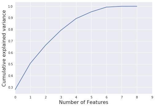
If you have low accuracy values for your Regression / Classification model, you could decide to stepwise remove the features with the lowest correlation, (or stepwise add features with the highest correlation).
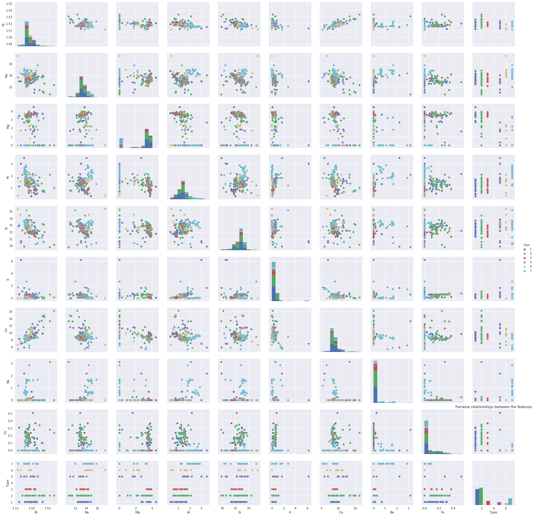
4.4 Pairwise relationships between the features
In addition to the correlation matrix, you can plot the pairwise relationships between the features, to see how these features are correlated.
|
1 2 3 |
ax = sns.pairplot(df_glass, hue='Type') plt.title('Pairwise relationships between the features') plt.show() |
5. Final Words
In my opinion, the best way to master the scikit-learn library is to simply start coding with it. I hope this blog-post gave some insight into the working of scikit-learn library, but for the ones who need some more information, here are some useful links:
dataschool – machine learning with scikit-learn video series
Classification example using the iris dataset
Official scikit-learn documentation
14 gedachten over “Classification with Scikit-Learn”
2.3 Classification and validation
def get_train_test(df, y_col, ratio):
mask = np.random.rand(len(df)) < ratio
What is < ratio
When I run this , i get the following error
NameError: name ‘lt’ is not defined
Ahmet bey harika bir yazı olmuş, elinize sağlık . Çok istifade ettim
Tesekkurler!
Hi Ahmet,
thanks for your examples. We used it for educational purposes, however please revisit the section where you transform non-numerical values to numerical values.
If I understand you correctly, you run correlations on numerical values which do not have any ‘numerical meaning’ but are strictly categorical (‘glass type’); the results (other than ‘ 0’) therefore are arbitrary and strongly depend only on the ordering of the types.
Hi Simon,
Thanks for the feedback! I’ll update it as soon as I have time.
Hi Simon,
The correlation matrix was actually made on the glass dataset, which does not contain any categorical data. But I did use this opportunity to update the code and explicitly mention the dangers of one-hot encoding categorical data, and also added a few additional sections.
Great article! I like the useful plots. How could you perform feature subset selection based on groups of subsets that have to be considered together? (Where a single feature is FeatureHashed to a fixed size vector). Do you have any resources for this case?
Merhaba hocam elinize sağlık. Benim sorunum şu. Predict yaparken 3 saat falan bekliyor acaba nedeni RAM in yetmediğinden mi ?
Merhaba Baris, predict yaparkene mi fit yaparkene mi uzun suruyor? Uzun surmesinin bir koc sebebi olabilir ama daha fazla RAM herzaman iyidir
Hi Ahmet,
Thanks for another very informative post, I think I’ve learned more from your tutorials than my college lecturers! One question that came up here and in one of my projects was how to generate correlation matrices with both categorical & numerical data? How would you approach this in the binary and multi-class case?
Hi Liam,
Thank you for the compliment.
What I usually do with categorical data is as follows; If the number of categorical values for a specific column is too large (lets say > 50) I LabelEncode it. Here the number of columns remains the same since each categorical value is encoded into a numerical value.
If the number of categorical values in a specific column is not too large, I OneHote Encode that column. This is described in section 3.3
Hello,
Why don’t you use sklearn.model_selection.train_test_split?
Thanks!
That is a good question.
This is an old post, either I was not aware of train_test_split of sklearn at that time or wanted to code it myself 🙂